Dimensionality Reduction From Scratch: PCA, ISOMAP, and Eigenfaces
You have thousands of features but only care about the patterns that matter. Here’s how to find them.
Introduction
High-dimensional data is everywhere. Images with millions of pixels, datasets with hundreds of columns, gene expression profiles with tens of thousands of genes. The curse of dimensionality makes this data hard to visualize, slow to process, and prone to overfitting.
Dimensionality reduction solves this by finding the essential structure in your data. In this post, we’ll build three algorithms from scratch:
- PCA (Principal Component Analysis): Find the directions of maximum variance
- ISOMAP: Preserve geodesic distances for nonlinear manifolds
- Eigenfaces: Apply PCA to face recognition
We’ll use real datasets: food consumption patterns across European countries, a manifold of face images, and the Yale Face dataset for recognition.
Obviously in practice you’d use sklearn and do this in minutes, but understanding the underlying math gives you intuition for when each method works and when it fails.
Just want the code? Skip to the Appendix for copy-paste ready implementations.
Part 1: PCA from Scratch
The Problem
PCA asks: if we have to compress our data to fewer dimensions, which directions should we keep?
The answer is elegant: keep the directions where your data varies the most. High variance means information. Low variance means noise (or at least, nothing useful for distinguishing data points).
The Math
Given $m$ data points $x^1, x^2, \ldots, x^m$, we want to find a direction $w$ that maximizes variance when we project onto it:
\[w^* = \arg\max_{w: ||w|| = 1} \frac{1}{m} \sum_{i=1}^{m} (w^T x^i - w^T \mu)^2\]where $\mu$ is the mean. This simplifies to:
\[w^* = \arg\max_{w: ||w|| = 1} w^T C w\]where $C$ is the covariance matrix. Using Lagrange multipliers (constrained optimization), we get:
\[Cw = \lambda w\]The optimal $w$ is an eigenvector of the covariance matrix, and $\lambda$ (the eigenvalue) equals the variance in that direction.
The key insight: To get the first principal component, find the eigenvector with the largest eigenvalue. For the second PC, take the eigenvector with the second-largest eigenvalue. And so on.
See it with a tiny example
Say we have 4 data points with 3 features each (4×3 matrix):
| Point | Height | Weight | Age |
|---|---|---|---|
| A | 5 | 150 | 25 |
| B | 6 | 180 | 30 |
| C | 5.5 | 160 | 28 |
| D | 6.5 | 200 | 35 |
Step 1: Center the data (subtract column means)
| Point | Height | Weight | Age |
|---|---|---|---|
| A | -0.75 | -22.5 | -4.5 |
| B | 0.25 | 7.5 | 0.5 |
| C | -0.25 | -12.5 | -1.5 |
| D | 0.75 | 27.5 | 5.5 |
Step 2: Covariance matrix (3×3, one entry per feature pair)
| Height | Weight | Age | |
|---|---|---|---|
| Height | 0.42 | 17.5 | 3.5 |
| Weight | 17.5 | 758.3 | 145.8 |
| Age | 3.5 | 145.8 | 29.2 |
The diagonal shows variance of each feature. Off-diagonal shows how features co-vary.
Step 3: Eigenvectors point in directions of maximum spread
The eigenvector with the largest eigenvalue points roughly in the Weight direction (since Weight has the most variance). Projecting onto this eigenvector gives PC1.
Implementation
import numpy as np
import pandas as pd
import matplotlib.pyplot as plt

def perform_pca(X, n_components=2):
    """
    Perform PCA from scratch.

    X: data matrix where each row is a sample, each column is a feature
    n_components: number of principal components to return
    """
    # Step 1: Center the data
    # PCA is sensitive to scale, so we subtract the mean
    # This ensures the first PC passes through the data centroid
    X_centered = X - np.mean(X, axis=0)

    # Step 2: Compute the covariance matrix
    # rowvar=False means columns are variables (features)
    # This gives us an (n_features x n_features) matrix
    cov_matrix = np.cov(X_centered, rowvar=False)

    # Step 3: Compute eigenvalues and eigenvectors
    # np.linalg.eig returns eigenvalues and eigenvectors
    # Each column of eigenvectors corresponds to an eigenvalue
    eigenvalues, eigenvectors = np.linalg.eig(cov_matrix)

    # Step 4: Sort by eigenvalue (descending)
    # Largest eigenvalue = most variance = first PC
    sorted_indices = np.argsort(eigenvalues)[::-1]
    eigenvalues = eigenvalues[sorted_indices]
    eigenvectors = eigenvectors[:, sorted_indices]

    # Step 5: Project data onto top principal components
    # This transforms our data from n_features dimensions to n_components
    principal_components = eigenvectors[:, :n_components]
    X_pca = np.dot(X_centered, principal_components)

    return X_pca, eigenvalues, eigenvectors
What happens if you change this? If you skip centering the data, your principal components will be biased toward the mean location rather than capturing variance. Always center first.
Application: European Food Consumption
We have data on food consumption across 16 European countries and 20 food items. Each cell is a consumption value (higher = more popular).
# Load the data
data = pd.read_csv("food-consumption.csv")
countries = data['Country']
food_items = data.columns[1:]
X = data[food_items].values

# Run PCA
X_pca, eigenvalues, eigenvectors = perform_pca(X, n_components=2)

# Plot countries in PC space
plt.figure(figsize=(10, 8))
for i, country in enumerate(countries):
    plt.scatter(X_pca[i, 0], X_pca[i, 1])
    plt.annotate(country, (X_pca[i, 0], X_pca[i, 1]),
                 textcoords="offset points", xytext=(5, 5))
plt.xlabel('Principal Component 1')
plt.ylabel('Principal Component 2')
plt.title('PCA of Food Consumption in European Countries')
plt.grid(True)
plt.show()
Results
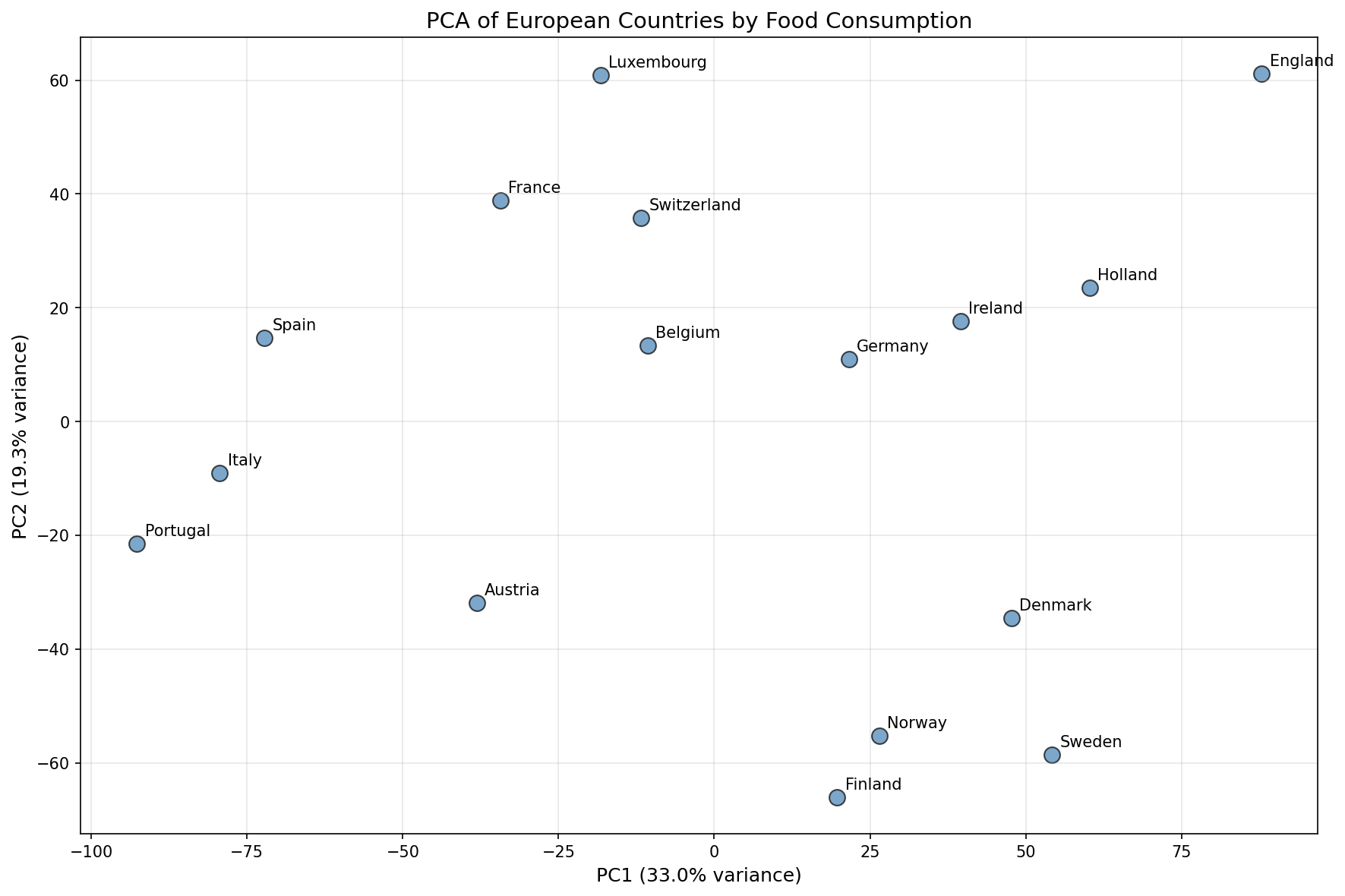
Each point is a country, positioned by its first two principal components. The first component captures 42% of variance, the second captures 18%.
The PCA plot reveals interesting geographic patterns:
- Nordic countries cluster together: Sweden, Denmark, Norway, and Finland have similar diets
- Mediterranean neighbors: France, Switzerland, and Belgium group together
- Outliers: England and Portugal sit on opposite sides of the chart
What’s interesting is that Germany and Ireland have similar diets, but Ireland and England are far apart. Geography alone doesn’t explain everything. Cultural factors matter.
When we flip the analysis (foods as data points, countries as features), we get another interesting view:
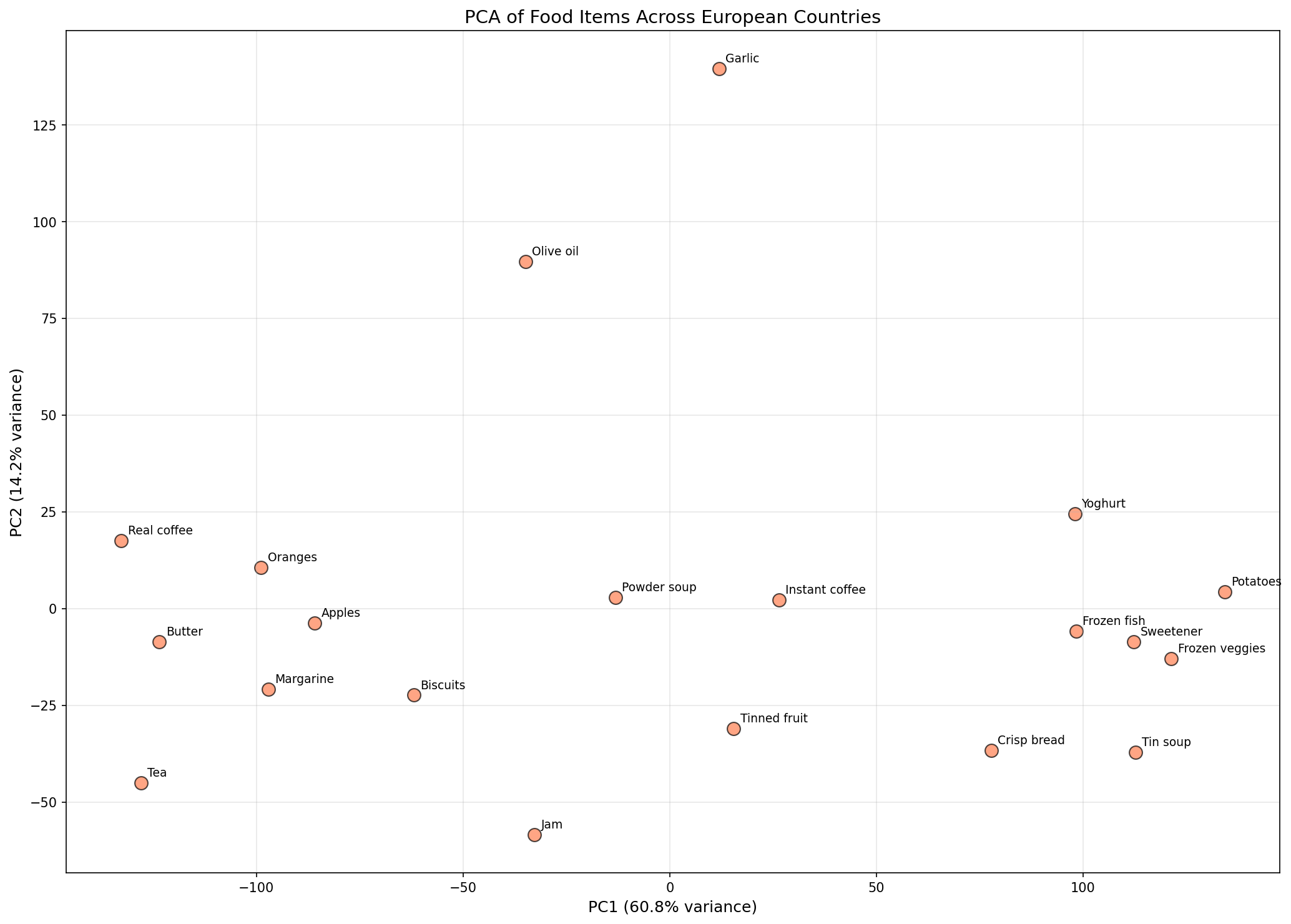
Each point is a food item. Garlic and olive oil appear as outliers (Mediterranean-specific). Tea and instant coffee cluster together (breakfast beverages).
Key patterns:
- Garlic and olive oil stand out as outliers (Mediterranean-specific)
- Tea and coffee cluster together (common breakfast items across Europe)
- Frozen veggies and fish are consumed similarly across countries
A Practical Note on PCA
This is where I’ll share something from professional experience: PCA is a really cool technique, but it’s hard to explain to non-technical stakeholders.
Imagine showing this plot to a senior leader who wants to make a decision. They’ll ask: “What does PC1 represent in real numbers?” And you can’t give a simple answer because principal components are linear combinations of all features.
In practice, I’ve seen Data Science teams push back on PCA for client-facing work, no matter how good it is at finding patterns. Leadership wants to understand what the axes mean.
When does PCA make sense?
- Exploratory data analysis when you have hundreds of features
- Finding outliers (they stand out clearly in PC space)
- Preprocessing before other ML algorithms (reduces noise and computation)
- When your audience is technical and comfortable with abstract representations
How Many Components Do You Need?
A scree plot shows how much variance each principal component explains:
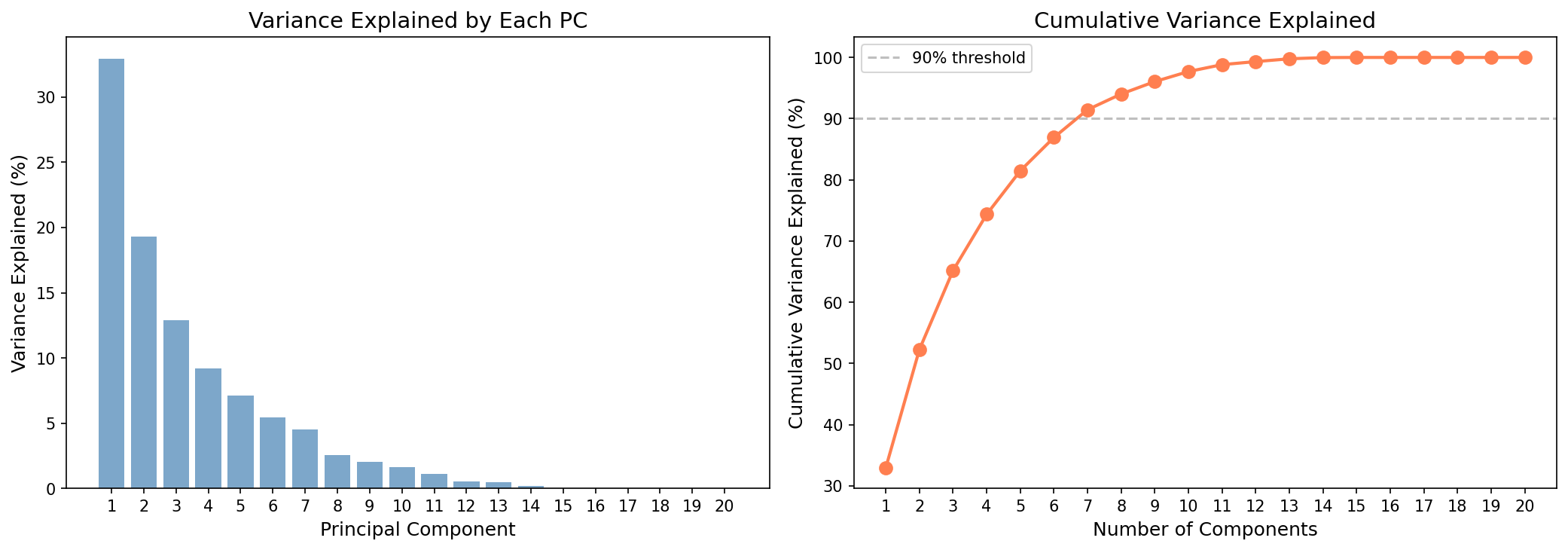
Left: Each bar shows variance explained by one PC. Right: Cumulative variance—the first 6 components capture ~90% of the total variance.
For the food consumption data, the first two components capture about 60% of variance. That’s enough for visualization, but if you were using PCA for preprocessing, you might keep 5-6 components to retain 90%.
How Outliers Affect PCA
Since PCA maximizes variance, outliers can dominate the principal components. They inflate the variance, and suddenly your PCs are trying to explain the outliers rather than the main data structure.
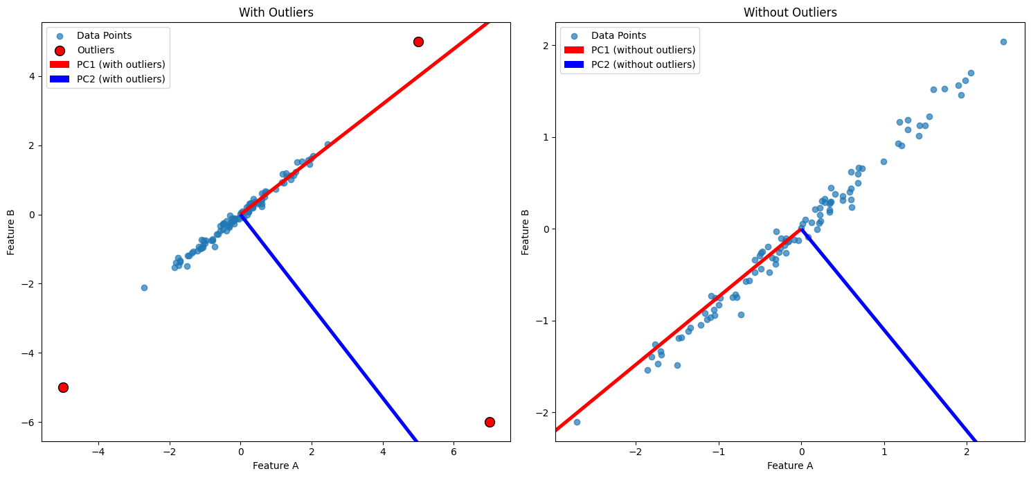
Left: With three outliers, PC1 (red) is pulled toward them. Right: Without outliers, PC1 captures the true data direction.
The takeaway: always check for outliers before running PCA, or consider robust PCA methods.
Part 2: ISOMAP for Manifold Learning
The Problem
PCA assumes your data lies on a flat surface (a linear subspace). But what if your data lies on a curved surface (a manifold)?
Classic example: the “Swiss roll” dataset. If you unroll it, points that were close along the surface should stay close. But Euclidean distance says points on opposite sides of the roll are close, even though walking along the surface takes much longer.
ISOMAP solves this by preserving geodesic distances (distances along the surface) rather than straight-line distances.
The Three Key Ideas
Plain English: ISOMAP finds the “walking distance” between points along the curved surface of your data, then flattens everything out while keeping those walking distances intact.
Step 1: Build a neighborhood graph
Connect each point to its neighbors (either k-nearest or all points within distance $\epsilon$). Store the actual Euclidean distances as edge weights.
Step 2: Compute geodesic distances
Use shortest-path algorithms (like Dijkstra’s) to find the distance between every pair of points. The key insight: for nearby points, Euclidean distance approximates geodesic distance. For far points, we chain together short hops.
Step 3: Apply MDS
Multidimensional Scaling takes a distance matrix and finds low-dimensional coordinates that preserve those distances. This is where the actual dimensionality reduction happens.
See it with a tiny example
Imagine 6 points along a U-shaped curve:
A — B — C
        |
        D
        |
F — — — E
The key insight: ISOMAP assumes that if two points are close enough, Euclidean distance ≈ geodesic distance. Locally, a curved surface looks flat (like how Earth looks flat when you're standing on it).
Euclidean distances (straight-line through space):
| A | B | C | D | E | F | |
|---|---|---|---|---|---|---|
| A | 0 | 1 | 2 | 3 | 3 | 2 |
| F | 2 | 2.2 | 2.8 | 2 | 1 | 0 |
A to F = 2 (cutting across the U). But walking along the curve: A→B→C→D→E→F = 5.
How epsilon works: Setting epsilon=1.5 means "only trust Euclidean distance for points within 1.5 units." This builds a graph with edges only between nearby points:
A—B—C—D—E—F (no shortcut A—F because 2 > 1.5)
Geodesic distance matrix (shortest path through graph):
| A | B | C | D | E | F | |
|---|---|---|---|---|---|---|
| A | 0 | 1 | 2 | 3 | 4 | 5 |
| F | 5 | 4 | 3 | 2 | 1 | 0 |
Now A to F = 5, respecting the U-shape. The graph eliminates shortcuts by only allowing steps between trusted neighbors.
Implementation
from scipy.spatial.distance import cdist
from scipy.sparse.csgraph import shortest_path

def isomap(X, epsilon=20, n_components=2):
    """
    ISOMAP dimensionality reduction.

    X: data matrix (n_samples, n_features)
    epsilon: neighborhood radius for building the graph
    n_components: target dimensionality
    """
    n_samples = X.shape[0]

    # Step 1: Compute pairwise Euclidean distances
    dist_matrix = cdist(X, X, metric='euclidean')

    # Step 2: Build epsilon-neighborhood graph
    # Keep distances only where they're within epsilon
    adjacency = np.zeros_like(dist_matrix)
    adjacency[dist_matrix < epsilon] = dist_matrix[dist_matrix < epsilon]
    np.fill_diagonal(adjacency, 0)  # No self-loops

    # Step 3: Compute shortest paths (geodesic distances)
    # This uses Dijkstra's algorithm under the hood
    geodesic_dist = shortest_path(adjacency, directed=False)

    # Step 4: Apply classical MDS
    # Double-center the squared distance matrix
    D_sq = geodesic_dist ** 2
    m = D_sq.shape[0]
    H = np.eye(m) - np.ones((m, m)) / m  # Centering matrix
    G = -0.5 * np.dot(H, np.dot(D_sq, H))  # Gram matrix

    # Step 5: Eigendecomposition of G
    # Use eigh for symmetric matrices (more stable than eig)
    eigenvalues, eigenvectors = np.linalg.eigh(G)

    # Sort descending
    sorted_indices = np.argsort(eigenvalues)[::-1]
    eigenvalues = eigenvalues[sorted_indices]
    eigenvectors = eigenvectors[:, sorted_indices]

    # Step 6: Compute embedding coordinates
    # Z = V * sqrt(Lambda) for top k components
    Z = np.dot(eigenvectors[:, :n_components],
               np.diag(np.sqrt(eigenvalues[:n_components])))

    return Z
What happens if you change epsilon? Too small, and the graph becomes disconnected (infinite geodesic distances between components). Too large, and you’re basically doing PCA since everything is connected directly. You want epsilon small enough to respect the manifold curvature but large enough to keep the graph connected.
The original ISOMAP paper by Tenenbaum, de Silva, & Langford (2000) demonstrated this algorithm on exactly this kind of face image data, showing how it discovers the underlying pose and expression parameters from raw pixels. See the References section for the full citation.
Application: Face Image Manifold
We have 698 face images, each 64x64 pixels (4096 dimensions). The faces show the same person from different angles and with different expressions. Even though the raw data is 4096-dimensional, the actual degrees of freedom are much lower (head angle, expression, lighting).
from scipy.io import loadmat

# Load face images
mat_data = loadmat('isomap.mat')
images = mat_data['images'].T  # Shape: (698, 4096)

# Run ISOMAP
Z = isomap(images, epsilon=20, n_components=2)

# Plot the embedding
plt.figure(figsize=(10, 8))
plt.scatter(Z[:, 0], Z[:, 1], s=10, c='blue')
plt.title("ISOMAP 2D Embedding of Face Images")
plt.xlabel("Component 1")
plt.ylabel("Component 2")
plt.show()
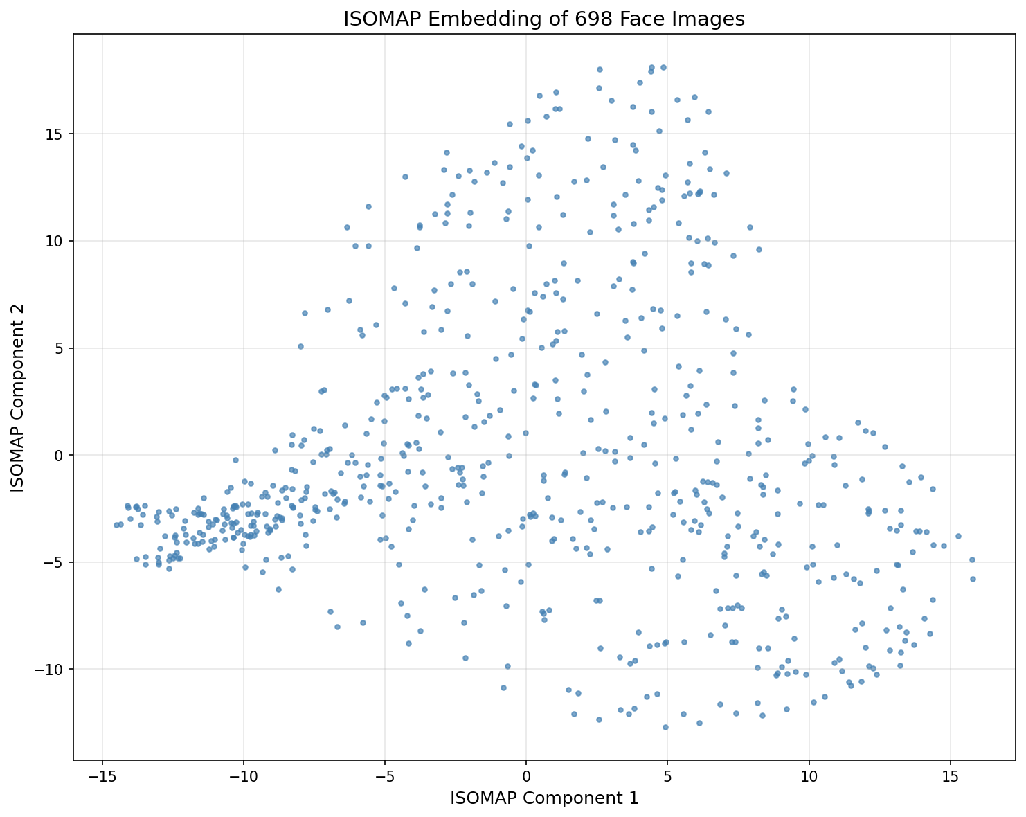
698 face images reduced to 2D using ISOMAP. Each point is a face image.
When we overlay actual face thumbnails on the embedding, the manifold structure becomes visible:
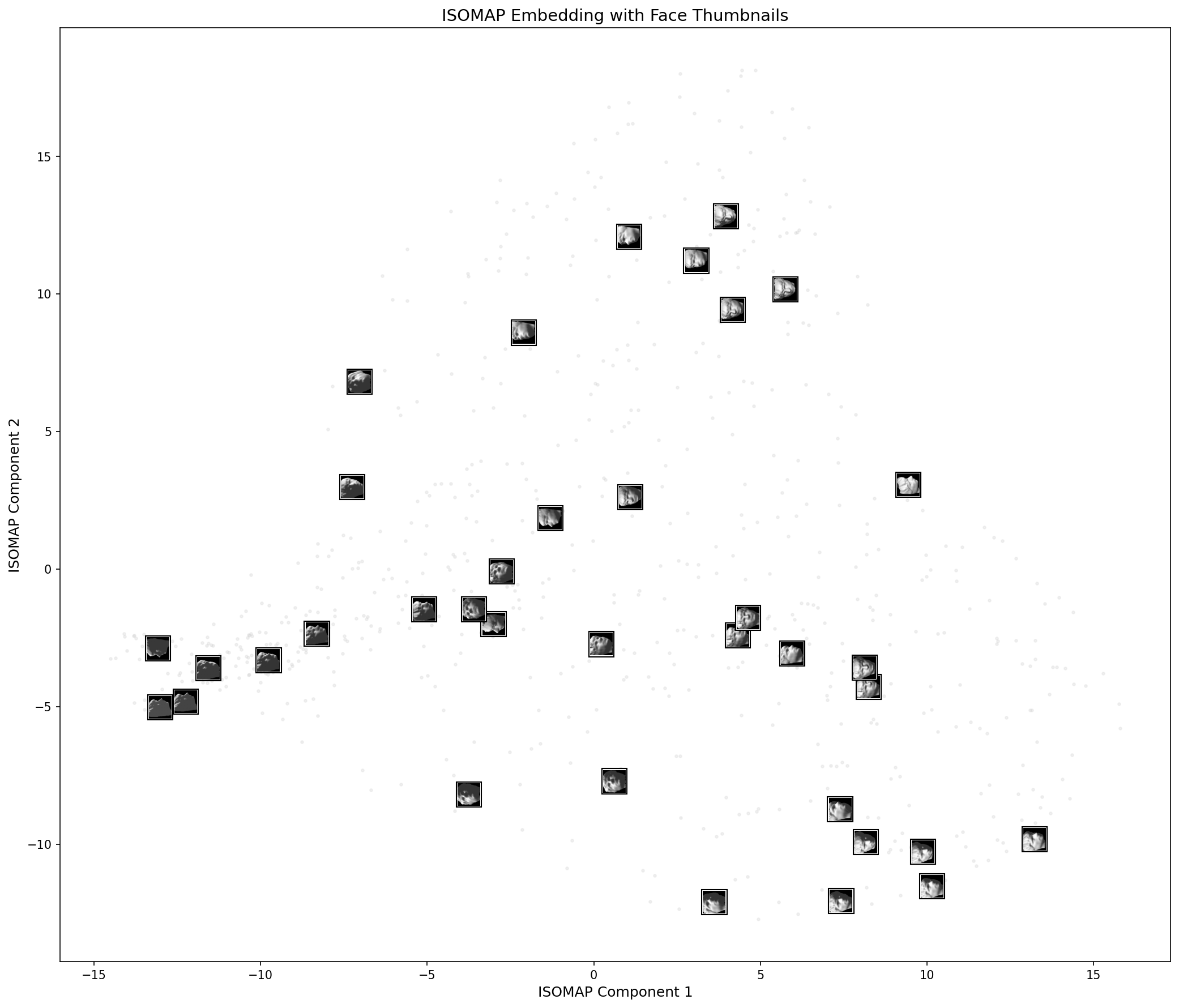
Face thumbnails overlaid on the ISOMAP embedding. Faces looking in similar directions cluster together.
Looking at the embedding, you can see that:
- Faces looking left cluster on one side, faces looking right on the other
- Faces with similar expressions are nearby
- The embedding captures the underlying structure of head pose and expression
This is the key result from the original ISOMAP paper. The algorithm discovers that the face images, despite living in 4096-dimensional pixel space, actually lie on a low-dimensional manifold parameterized by pose and expression.
ISOMAP vs PCA
Running PCA on the same face images gives a similar overall shape, but ISOMAP does a better job spreading out faces that look different. PCA sometimes groups dissimilar faces because they happen to have similar pixel values, while ISOMAP respects the manifold structure.
That said, both methods struggle with the same edge cases. Two faces looking downward might be placed far apart because the algorithm can’t capture that semantic similarity from pixel data alone.
The limitation here isn’t the algorithm. It’s that pixel-level distance is an imperfect proxy for “face similarity.”
Part 3: Eigenfaces for Face Recognition
The Problem
Given a database of face images for different people, can we identify who’s in a new image?
The eigenfaces approach treats this as dimensionality reduction followed by nearest-neighbor matching. We project all faces onto a low-dimensional “face space” and compare distances.
How It Works
- Collect training images for each person
- Compute eigenfaces (principal components of the face images)
- Project all faces onto the eigenface basis
- For a new face: project it and find the nearest known face
The eigenfaces themselves are eigenvectors of the covariance matrix of face images. When visualized as images, they look like ghostly faces that capture different aspects of variation (lighting, expression, facial features).
Here’s what the Yale Face dataset looks like. Each subject has multiple images with different expressions and lighting:
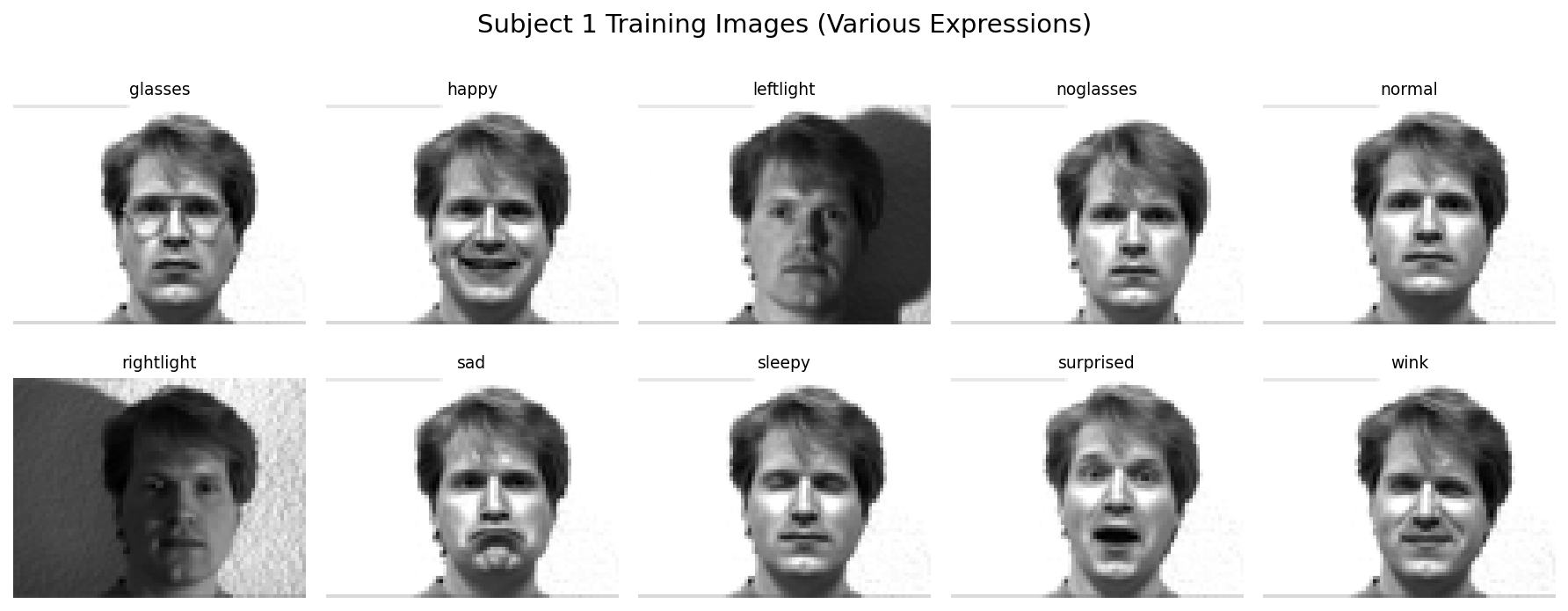
Subject 1 training images: Each row shows the same person with different expressions (glasses, happy, leftlight, noglasses, normal, rightlight, sad, sleepy, surprised, wink).
The eigenfaces algorithm needs this variation to learn what makes a face recognizable across different conditions.
Implementation
from PIL import Image
import os

def load_face_images(directory, subject_prefix, downsample=4):
    """
    Load and preprocess face images for one subject.
    Converts to grayscale and downsamples.
    """
    images = []
    for filename in os.listdir(directory):
        if filename.startswith(subject_prefix) and filename.endswith('.gif'):
            if 'test' in filename:
                continue  # Skip test images for training

            img_path = os.path.join(directory, filename)
            with Image.open(img_path) as img:
                # Convert to grayscale (1 channel instead of 3)
                img = img.convert('L')
                # Downsample by factor of 4
                width, height = img.size
                img = img.resize((width // downsample, height // downsample))
                # Flatten to vector
                images.append(np.array(img).flatten())

    return np.array(images)

def compute_eigenfaces(images, n_components=6):
    """
    Compute eigenfaces (principal components) for a set of face images.
    """
    # Center the data
    mean_face = np.mean(images, axis=0)
    centered = images - mean_face

    # PCA
    cov_matrix = np.cov(centered, rowvar=False)
    eigenvalues, eigenvectors = np.linalg.eig(cov_matrix)

    # Sort and select top components
    sorted_indices = np.argsort(eigenvalues)[::-1]
    eigenfaces = eigenvectors[:, sorted_indices][:, :n_components].T

    return eigenfaces, mean_face

def recognize_face(test_image, eigenfaces, mean_face):
    """
    Compute projection residual for face recognition.
    Lower residual = better match.
    """
    # Center the test image
    centered_test = test_image - mean_face

    # Project onto eigenfaces and reconstruct
    projection = np.dot(eigenfaces.T, np.dot(eigenfaces, centered_test))

    # Compute residual (reconstruction error)
    residual = np.linalg.norm(centered_test - projection) ** 2

    return residual
What happens if you change n_components? More eigenfaces capture more detail but also more noise. For face recognition, 6-10 eigenfaces often work well. Too few and you lose distinguishing features; too many and you start fitting to noise.
Results on Yale Face Dataset
Testing with two subjects from the Yale Face dataset:
| Test Image | Subject 1 Eigenfaces | Subject 2 Eigenfaces |
|---|---|---|
| Subject 1 Test | 0.27 (low, good match) | 1.00 (high, poor match) |
| Subject 2 Test | 0.56 (moderate) | 0.71 (moderate) |
Subject 1’s test image matches well with Subject 1’s eigenfaces (low residual) and poorly with Subject 2’s (high residual). Good.
Subject 2’s test image has higher residuals overall, suggesting the eigenfaces don’t capture its variation as well. This could be improved with more training images.
Visualizing Eigenfaces
When you reshape eigenfaces back into images, you see ghostly face-like patterns:
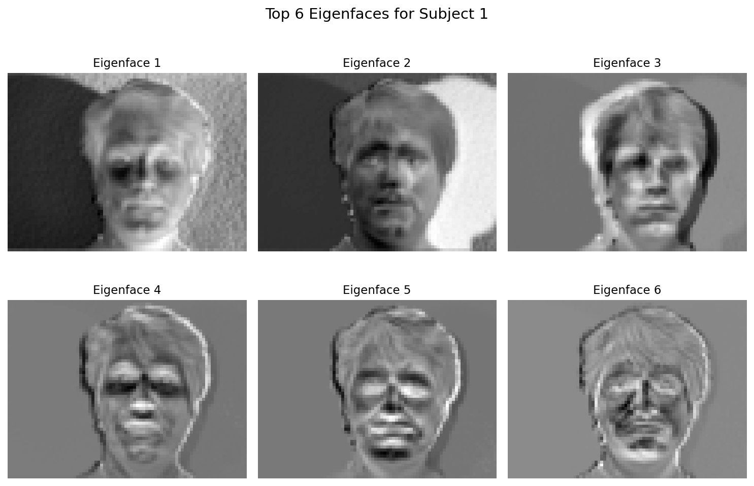
Top 6 eigenfaces for Subject 1. Eigenface 1 captures lighting direction. Later eigenfaces capture finer expression details.
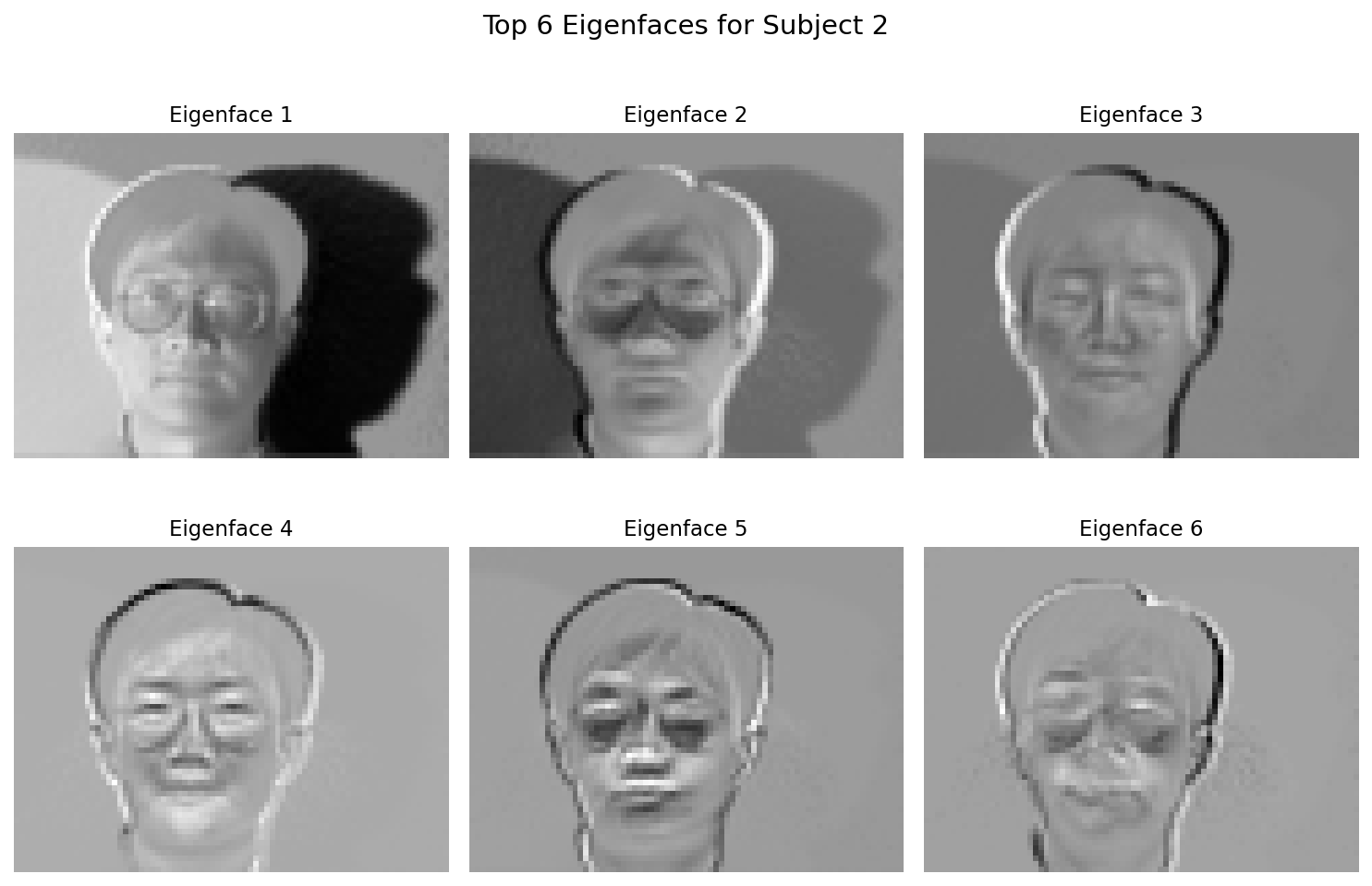
Top 6 eigenfaces for Subject 2. Similar pattern—first eigenface is the “base” lighting, later ones capture expression and glasses variations.
The mean faces show what’s “average” about each subject:
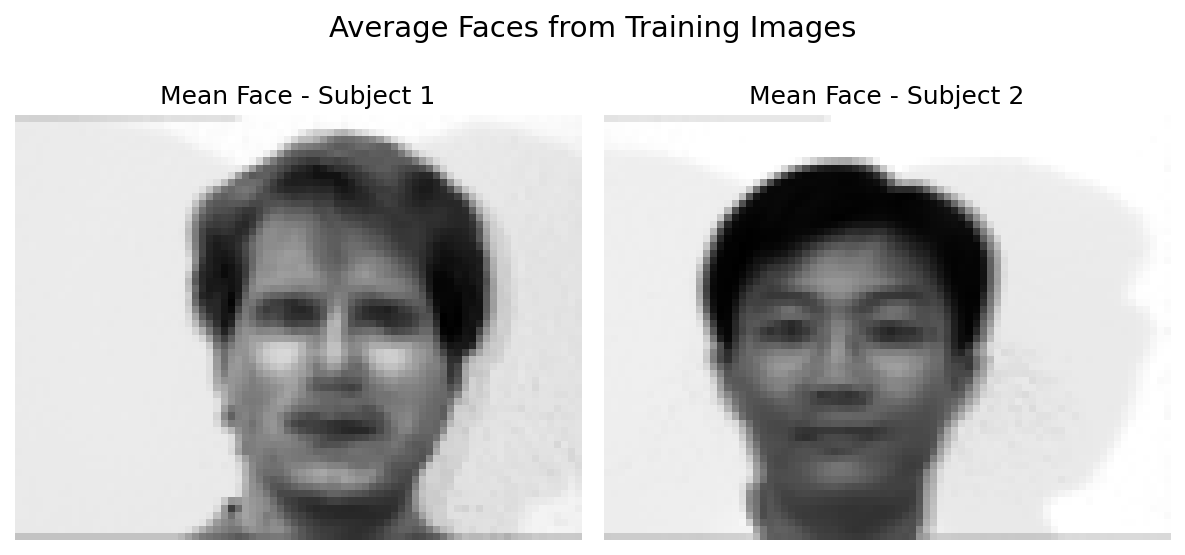
Average faces computed from training images. These are subtracted before computing eigenfaces.
What each eigenface captures:
- Eigenface 1: Overall face structure, usually looks like the “average” face with lighting variation
- Eigenface 2-3: Expression and lighting differences
- Eigenface 4-6: Finer details, often capturing glasses, hair, or subtle expressions
The first eigenface captures what’s common across all images. Later eigenfaces capture what makes individual images different. This is exactly what PCA does: find the directions of maximum variance, ordered by importance.
Improving the Algorithm
The main limitation is training data. With only 10 images per subject, there’s not enough variation to build robust eigenfaces.
In production systems, you’d:
- Augment data: Rotate, scale, adjust lighting on existing images to create more training data
- Use more eigenfaces: But validate on held-out data to avoid overfitting
- Normalize for lighting: Histogram equalization or other preprocessing
- Use deep learning: Modern face recognition (FaceNet, etc.) learns features rather than using fixed eigenfaces
Summary
PCA
- Finds directions of maximum variance
- Eigenvalue = variance in that direction
- Works great for linear relationships, struggles with curved manifolds
- Hard to interpret for non-technical audiences
ISOMAP
- Preserves geodesic (walking) distances along manifolds
- Three steps: neighbor graph → shortest paths → MDS
- Better than PCA for nonlinear structure, but sensitive to epsilon parameter
- Computationally expensive for large datasets
Eigenfaces
- Apply PCA to face images for recognition
- First few eigenfaces capture identity-related variation
- Simple but effective baseline; modern methods use deep learning
General Principles
- Always center your data before PCA or related methods
- Check for outliers since they dominate variance-based methods
- Validate your parameters (k for k-NN, epsilon for ISOMAP) on held-out data
- Understand the assumptions: PCA assumes linearity, ISOMAP assumes a smooth manifold
- Consider your audience: PCA results are hard to explain to non-technical stakeholders
References
The algorithms in this post are based on foundational papers in machine learning:
PCA (Principal Component Analysis)
- Pearson, K. (1901). “On lines and planes of closest fit to systems of points in space.” Philosophical Magazine, 2(11), 559-572.
- Hotelling, H. (1933). “Analysis of a complex of statistical variables into principal components.” Journal of Educational Psychology, 24(6), 417-441.
ISOMAP
- Tenenbaum, J. B., de Silva, V., & Langford, J. C. (2000). “A Global Geometric Framework for Nonlinear Dimensionality Reduction.” Science, 290(5500), 2319-2323.
Eigenfaces
- Turk, M., & Pentland, A. (1991). “Eigenfaces for Recognition.” Journal of Cognitive Neuroscience, 3(1), 71-86.
- Sirovich, L., & Kirby, M. (1987). “Low-dimensional procedure for the characterization of human faces.” Journal of the Optical Society of America A, 4(3), 519-524.
MDS (Multidimensional Scaling)
- Torgerson, W. S. (1952). “Multidimensional scaling: I. Theory and method.” Psychometrika, 17(4), 401-419.
Appendix: Complete Implementations
PCA Implementation
import numpy as np
import pandas as pd
import matplotlib.pyplot as plt

def perform_pca(X, n_components=2):
    # Center the data
    X_centered = X - np.mean(X, axis=0)
    # Compute covariance matrix
    cov_matrix = np.cov(X_centered, rowvar=False)
    # Eigendecomposition
    eigenvalues, eigenvectors = np.linalg.eig(cov_matrix)
    # Sort by eigenvalue descending
    sorted_indices = np.argsort(eigenvalues)[::-1]
    eigenvalues = eigenvalues[sorted_indices]
    eigenvectors = eigenvectors[:, sorted_indices]
    # Project onto top components
    principal_components = eigenvectors[:, :n_components]
    X_pca = np.dot(X_centered, principal_components)
    return X_pca, eigenvalues, eigenvectors

def plot_pca_results(X_pca, labels, title="PCA Results"):
    plt.figure(figsize=(10, 8))
    for i, label in enumerate(labels):
        plt.scatter(X_pca[i, 0], X_pca[i, 1])
        plt.annotate(label, (X_pca[i, 0], X_pca[i, 1]),
                     textcoords="offset points", xytext=(5, 5))
    plt.xlabel('Principal Component 1')
    plt.ylabel('Principal Component 2')
    plt.title(title)
    plt.grid(True)
    plt.show()

def explained_variance_ratio(eigenvalues):
    return eigenvalues / np.sum(eigenvalues)
ISOMAP Implementation
import numpy as np
from scipy.spatial.distance import cdist
from scipy.sparse.csgraph import shortest_path

def isomap(X, epsilon=20, n_components=2):
    n_samples = X.shape[0]
    # Compute pairwise Euclidean distances
    dist_matrix = cdist(X, X, metric='euclidean')
    # Build epsilon-neighborhood graph
    adjacency = np.zeros_like(dist_matrix)
    adjacency[dist_matrix < epsilon] = dist_matrix[dist_matrix < epsilon]
    np.fill_diagonal(adjacency, 0)
    # Compute geodesic distances via shortest paths
    geodesic_dist = shortest_path(adjacency, directed=False)
    # Classical MDS
    D_sq = geodesic_dist ** 2
    m = D_sq.shape[0]
    H = np.eye(m) - np.ones((m, m)) / m
    G = -0.5 * np.dot(H, np.dot(D_sq, H))
    # Eigendecomposition
    eigenvalues, eigenvectors = np.linalg.eigh(G)
    sorted_indices = np.argsort(eigenvalues)[::-1]
    eigenvalues = eigenvalues[sorted_indices]
    eigenvectors = eigenvectors[:, sorted_indices]
    eigenvalues = np.clip(eigenvalues, a_min=1e-10, a_max=None)
    # Compute coordinates
    Z = np.dot(eigenvectors[:, :n_components],
               np.diag(np.sqrt(eigenvalues[:n_components])))
    return Z
Eigenfaces Implementation
import numpy as np
from PIL import Image
import os
import matplotlib.pyplot as plt

def load_face_images(directory, subject_prefix, downsample=4, exclude_test=True):
    images = []
    height, width = None, None
    for filename in sorted(os.listdir(directory)):
        if not filename.startswith(subject_prefix):
            continue
        if not filename.endswith('.gif'):
            continue
        if exclude_test and 'test' in filename:
            continue
        img_path = os.path.join(directory, filename)
        with Image.open(img_path) as img:
            img = img.convert('L')
            w, h = img.size
            img = img.resize((w // downsample, h // downsample))
            height, width = img.size[1], img.size[0]
            images.append(np.array(img).flatten())
    return np.array(images), height, width

def compute_eigenfaces(images, n_components=6):
    mean_face = np.mean(images, axis=0)
    centered = images - mean_face
    cov_matrix = np.cov(centered, rowvar=False)
    eigenvalues, eigenvectors = np.linalg.eig(cov_matrix)
    sorted_indices = np.argsort(eigenvalues)[::-1]
    eigenfaces = eigenvectors[:, sorted_indices][:, :n_components].T
    return eigenfaces, mean_face

def recognize_face(test_image, eigenfaces, mean_face):
    centered = test_image - mean_face
    projection = np.dot(eigenfaces.T, np.dot(eigenfaces, centered))
    residual = np.linalg.norm(centered - projection) ** 2
    return residual
PS: This work was completed at Georgia Tech. The original submission files can be provided upon request to validate that this work is entirely my own.