Density Estimation and Mixture Models From Scratch
How do you estimate the shape of data when you don’t know what distribution it came from?
Introduction
Sometimes you have data but no idea what distribution generated it. Maybe it’s unimodal, maybe bimodal, maybe something weird. Histograms give you a rough picture, but they’re choppy and dependent on bin choices. What if you want a smooth, continuous estimate of the underlying density?
In this post, we build two approaches from scratch:
- Kernel Density Estimation (KDE): Place a smooth “bump” (kernel) at each data point and sum them up
- Gaussian Mixture Models (GMM): Assume the data comes from multiple Gaussian distributions and learn their parameters
We’ll also implement the Expectation-Maximization (EM) algorithm, the standard method for fitting GMMs when you don’t know which points belong to which component.
The applications: analyzing brain structure differences across political orientations (surprisingly interesting data), and classifying handwritten digits using GMM as a generative classifier.
Just want the code? Skip to the Appendix for copy-paste ready implementations.
Part 1: Histograms vs KDE
The Histogram Problem
Histograms are the most intuitive density estimate. Count how many points fall in each bin, normalize, done. But they have issues:
- Bin edges are arbitrary. Shift your bins slightly and the shape changes.
- Not smooth. Histograms are step functions. Real densities are usually smooth.
- Curse of dimensionality. In 2D you need bins squared, in 3D bins cubed. It gets sparse fast.
How KDE Works
Plain English: Instead of counting points in bins, we place a smooth “bump” centered at each data point. The density estimate at any location is the sum of all these bumps.
The formula:
\[\hat{f}(x) = \frac{1}{nh} \sum_{i=1}^{n} K\left(\frac{x - x_i}{h}\right)\]Where:
- $n$ is the number of data points
- $h$ is the bandwidth (controls how wide each bump is)
- $K$ is the kernel function (usually Gaussian)
- $x_i$ are your data points
The Gaussian kernel is:
\[K(u) = \frac{1}{\sqrt{2\pi}} e^{-\frac{u^2}{2}}\]See it with a tiny example
Say we have 3 data points: x = [2, 3, 5] and bandwidth h = 1.
To estimate density at x = 3:
- Distance from point 1: (3-2)/1 = 1 → K(1) ≈ 0.24
- Distance from point 2: (3-3)/1 = 0 → K(0) ≈ 0.40
- Distance from point 3: (3-5)/1 = -2 → K(-2) ≈ 0.05
Sum: (0.24 + 0.40 + 0.05) / (3 × 1) ≈ 0.23
The density is highest near the data points and smoothly decays away from them.
Implementation
import numpy as np
from scipy.stats import gaussian_kde

def kde_1d(data, bandwidth_factor=1.0):
    """
    Compute 1D kernel density estimate.

    Parameters:
    - data: 1D array of observations
    - bandwidth_factor: multiplier for Scott's rule bandwidth

    Returns:
    - kde: scipy gaussian_kde object
    """
    # scipy's gaussian_kde uses Scott's rule by default
    # h = n^(-1/5) * std(data)
    kde = gaussian_kde(data)

    # Adjust bandwidth if needed
    # bw_method scales the default bandwidth
    kde = gaussian_kde(data, bw_method=bandwidth_factor * kde.factor)

    return kde

def kde_2d(x, y, bandwidth_factor=1.0):
    """
    Compute 2D kernel density estimate.

    Parameters:
    - x, y: 1D arrays of coordinates
    - bandwidth_factor: multiplier for default bandwidth

    Returns:
    - kde: scipy gaussian_kde object for 2D data
    """
    # Stack into 2D array where each column is a point
    data = np.vstack([x, y])

    kde = gaussian_kde(data)
    kde = gaussian_kde(data, bw_method=bandwidth_factor * kde.factor)

    return kde
What happens if you change bandwidth? Too small, and you get a spiky estimate that overfits to individual points. Too large, and you oversmooth, missing real structure like multiple modes. Scott’s rule ($h = n^{-1/5} \cdot \sigma$) is a reasonable default, but you often need to tune it.
Choosing Bandwidth
There’s no perfect answer. Common approaches:
| Method | Formula | When to Use |
|---|---|---|
| Scott’s Rule | $h = n^{-1/5} \cdot \sigma$ | Default, assumes roughly Gaussian data |
| Silverman’s Rule | $h = 0.9 \cdot \min(\sigma, IQR/1.34) \cdot n^{-1/5}$ | More robust to outliers |
| Cross-validation | Minimize integrated squared error | When you need optimal bandwidth |
In practice, I start with Scott’s rule and adjust by eye. If the KDE looks too smooth (missing obvious peaks), decrease the bandwidth. If it’s too spiky, increase it.
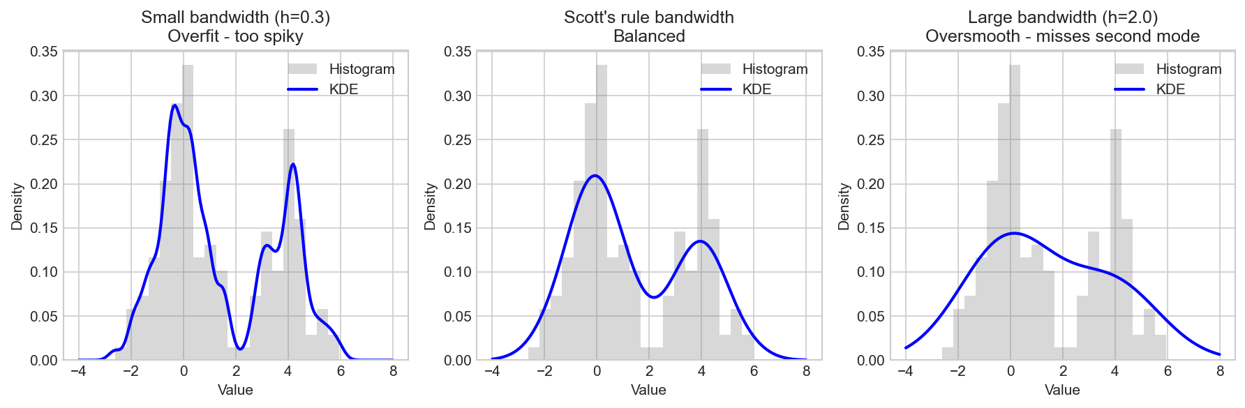 Left: Small bandwidth (h=0.3) shows spiky overfit. Middle: Scott’s rule bandwidth. Right: Large bandwidth (h=1.0) oversmooths and misses the second mode.
Histograms vs KDE: Trade-offs
| Aspect | Histogram | KDE |
|---|---|---|
| Interpretability | Easy (counts per bin) | Harder (smooth density) |
| Computation | Fast | Slower (scales with n) |
| Smoothness | Discontinuous | Continuous |
| Sampling | Can’t easily generate new points | Can sample from the density |
| High dimensions | Breaks down | Also struggles, but degrades more gracefully |
When to use histograms: Quick exploration, discrete data, when you need exact counts.
When to use KDE: Estimating continuous densities, generating synthetic data, when smoothness matters.
Part 2: Gaussian Mixture Models
The Problem with Single Gaussians
Sometimes your data has multiple clusters or modes. A single Gaussian can’t capture this. If you fit one Gaussian to bimodal data, you get a mean in the middle where no data actually lives.
Plain English: A GMM says “your data comes from K different Gaussian distributions, mixed together.” Each data point was generated by one of these Gaussians, but we don’t know which one.
The Model
A GMM with $K$ components has:
\[p(x) = \sum_{k=1}^{K} \pi_k \cdot \mathcal{N}(x \mid \mu_k, \Sigma_k)\]Where:
- $\pi_k$ is the mixing weight for component $k$. This is the probability that a randomly chosen point came from component $k$. All weights must sum to 1: $\sum_k \pi_k = 1$
- $\mu_k$ is the mean (center) of component $k$
- $\Sigma_k$ is the covariance matrix of component $k$, which controls the shape and orientation of the Gaussian
- $\mathcal{N}(x \mid \mu, \Sigma)$ is the multivariate Gaussian density function, which gives the probability density of observing $x$ given that it came from a Gaussian with mean $\mu$ and covariance $\Sigma$
See it with a tiny example
Setup: We have a GMM with K=2 components in 1D. Think of this as modeling data that comes from two different sources (like heights of men and women mixed together).
| Component | Weight π | Mean μ | Variance σ² | Interpretation |
|---|---|---|---|---|
| 1 | 0.6 | 0 | 1 | 60% of data, centered at 0 |
| 2 | 0.4 | 5 | 2 | 40% of data, centered at 5 |
Question: What's the probability density at x = 2?
Step 1: Compute each component's contribution.
For each component, we compute: (mixing weight) × (Gaussian density at x)
Component 1 contribution:
- Gaussian density at x=2 with μ=0, σ²=1: N(2 | 0, 1) = (1/√(2π)) × e^(-(2-0)²/2) = 0.054
- Weighted: π₁ × density = 0.6 × 0.054 = 0.032
Component 2 contribution:
- Gaussian density at x=2 with μ=5, σ²=2: N(2 | 5, 2) = (1/√(4π)) × e^(-(2-5)²/4) = 0.030
- Weighted: π₂ × density = 0.4 × 0.030 = 0.012
Step 2: Sum all contributions.
Total density: p(x=2) = 0.032 + 0.012 = 0.044
Interpretation: Even though x=2 is closer to component 1's mean (distance of 2) than component 2's mean (distance of 3), both components contribute to the density. Component 1 contributes more because it's both closer AND more common (weight 0.6 vs 0.4).
Why MLE Doesn’t Work Directly
For a single Gaussian, maximum likelihood estimation is straightforward. You take derivatives, set to zero, and get the sample mean and covariance.
For GMMs, the likelihood is:
\[L(\theta) = \prod_{i=1}^{n} \sum_{k=1}^{K} \pi_k \cdot \mathcal{N}(x_i \mid \mu_k, \Sigma_k)\]Taking the log:
\[\log L(\theta) = \sum_{i=1}^{n} \log \left[ \sum_{k=1}^{K} \pi_k \cdot \mathcal{N}(x_i \mid \mu_k, \Sigma_k) \right]\]The problem: that log of a sum doesn’t simplify nicely. We can’t separate terms and solve for each parameter independently. The sum is inside the log.
The solution: Expectation-Maximization (EM).
Part 3: The EM Algorithm
The Core Idea
EM alternates between two steps:
-
E-step (Expectation): Given current parameters, compute the probability that each point belongs to each component. These are called “responsibilities.”
-
M-step (Maximization): Given responsibilities, update the parameters (means, covariances, weights) to maximize the expected log-likelihood.
Repeat until convergence.
The Responsibility Formula
Using Bayes’ rule, the responsibility $\tau_k^i$ (probability that point $i$ belongs to component $k$) is:
\[\tau_k^i = \frac{\pi_k \cdot \mathcal{N}(x_i \mid \mu_k, \Sigma_k)}{\sum_{j=1}^{K} \pi_j \cdot \mathcal{N}(x_i \mid \mu_j, \Sigma_j)}\]Let’s break this formula down piece by piece:
The numerator $\pi_k \cdot \mathcal{N}(x_i \mid \mu_k, \Sigma_k)$ asks: “What’s the probability that this point came from component $k$?”
- $\pi_k$ is how common component $k$ is overall (its mixing weight)
- $\mathcal{N}(x_i \mid \mu_k, \Sigma_k)$ is how well point $x_i$ fits component $k$’s Gaussian distribution
- Multiplying them gives: “probability of picking component $k$” × “probability of seeing this point given component $k$”
The denominator $\sum_{j=1}^{K} \pi_j \cdot \mathcal{N}(x_i \mid \mu_j, \Sigma_j)$ is the total probability of observing $x_i$ under the entire mixture model. We sum over all $K$ components.
The ratio normalizes everything so that the responsibilities for point $i$ sum to 1 across all components: $\sum_{k=1}^{K} \tau_k^i = 1$.
This is just Bayes’ rule. We’re computing: $P(\text{component } k \mid \text{point } x_i)$.
See it with a tiny example
Setup: We have a 2-component GMM with these parameters:
| Component | Weight π | Mean μ | Variance σ² |
|---|---|---|---|
| 1 | 0.6 | 0 | 1 |
| 2 | 0.4 | 5 | 2 |
Where do these numbers come from? We set them up for this example. Component 1 is centered at 0 and accounts for 60% of the data (π₁ = 0.6). Component 2 is centered at 5 and accounts for 40% (π₂ = 0.4).
Question: For a new point x = 2, what's the probability it came from each component?
Step 1: Compute the Gaussian density for each component.
The 1D Gaussian formula is: N(x | μ, σ²) = (1/√(2πσ²)) × exp(-(x-μ)²/(2σ²))
For component 1 (μ₁ = 0, σ₁² = 1):
- Distance from mean: (x - μ₁)² = (2 - 0)² = 4
- Exponent: -4 / (2 × 1) = -2
- Density: (1/√(2π)) × e⁻² = 0.399 × 0.135 = 0.054
For component 2 (μ₂ = 5, σ₂² = 2):
- Distance from mean: (x - μ₂)² = (2 - 5)² = 9
- Exponent: -9 / (2 × 2) = -2.25
- Density: (1/√(4π)) × e⁻²·²⁵ = 0.282 × 0.105 = 0.030
Step 2: Multiply each density by its mixing weight.
- Component 1: π₁ × N(2|0,1) = 0.6 × 0.054 = 0.032
- Component 2: π₂ × N(2|5,2) = 0.4 × 0.030 = 0.012
Step 3: Compute the denominator (sum over all components).
Total = 0.032 + 0.012 = 0.044
Step 4: Divide to get responsibilities.
| Component | Numerator (π × N) | Responsibility τ |
|---|---|---|
| 1 | 0.032 | 0.032 / 0.044 = 0.73 |
| 2 | 0.012 | 0.012 / 0.044 = 0.27 |
Interpretation: Point x = 2 has 73% responsibility to component 1 and 27% to component 2. This makes sense: x = 2 is closer to component 1's mean (0) than to component 2's mean (5), and component 1 is more common overall (60% vs 40%).
Notice the responsibilities sum to 1: 0.73 + 0.27 = 1.0 ✓
The M-Step Updates
Given responsibilities from the E-step, we now update all parameters. The key insight: these are just weighted versions of the formulas you already know for mean and variance, where each point is weighted by how much it “belongs” to that component.
Step 1: Effective count for component $k$
\[N_k = \sum_{i=1}^{n} \tau_k^i\]This sums all responsibilities for component $k$ across all $n$ data points. If we have 100 points and component 1 has average responsibility 0.6 per point, then $N_1 \approx 60$. This tells us “how many points effectively belong to this component.”
Step 2: Updated mixing weights
\[\pi_k = \frac{N_k}{n}\]The new weight for component $k$ is simply what fraction of the data (in terms of responsibility) belongs to it. If $N_k = 60$ out of $n = 100$ points, then $\pi_k = 0.6$.
Step 3: Updated means
\[\mu_k = \frac{1}{N_k} \sum_{i=1}^{n} \tau_k^i \cdot x_i\]This is a weighted average of all data points, where the weight for point $i$ is its responsibility $\tau_k^i$. Points that strongly belong to component $k$ (high $\tau_k^i$) pull the mean toward them. Points that barely belong (low $\tau_k^i$) have little influence.
Step 4: Updated covariances
\[\Sigma_k = \frac{1}{N_k} \sum_{i=1}^{n} \tau_k^i (x_i - \mu_k)(x_i - \mu_k)^T\]Same idea: weighted average of squared deviations from the mean. The $(x_i - \mu_k)(x_i - \mu_k)^T$ term computes the outer product (giving a matrix), and we weight each by responsibility.
See it with a tiny example
Setup: We have 4 data points in 1D and K=2 components. After running the E-step, here are the responsibilities:
| Point xᵢ | Value | τ₁ (component 1) | τ₂ (component 2) |
|---|---|---|---|
| 1 | 1.0 | 0.9 | 0.1 |
| 2 | 2.0 | 0.8 | 0.2 |
| 3 | 8.0 | 0.2 | 0.8 |
| 4 | 9.0 | 0.1 | 0.9 |
Step 1: Compute effective counts.
- N₁ = 0.9 + 0.8 + 0.2 + 0.1 = 2.0
- N₂ = 0.1 + 0.2 + 0.8 + 0.9 = 2.0
Step 2: Update weights.
- π₁ = 2.0 / 4 = 0.5
- π₂ = 2.0 / 4 = 0.5
Step 3: Update means.
- μ₁ = (1/2.0) × (0.9×1 + 0.8×2 + 0.2×8 + 0.1×9) = 4.9/2.0 = 2.45
- μ₂ = (1/2.0) × (0.1×1 + 0.2×2 + 0.8×8 + 0.9×9) = 15.0/2.0 = 7.50
Interpretation: Component 1's mean (2.45) is pulled toward points 1 and 2 (which have high responsibility to it). Component 2's mean (7.50) is pulled toward points 3 and 4.
Implementation
import numpy as np
from scipy.stats import multivariate_normal

def em_gmm(X, K, max_iters=100, tol=1e-6, seed=None):
    """
    Fit a Gaussian Mixture Model using EM algorithm.

    Parameters:
    - X: data matrix (n_samples, n_features)
    - K: number of components
    - max_iters: maximum iterations
    - tol: convergence tolerance for log-likelihood
    - seed: random seed for initialization

    Returns:
    - pi: mixing weights (K,)
    - mu: means (K, n_features)
    - Sigma: covariances (K, n_features, n_features)
    - responsibilities: final responsibilities (n_samples, K)
    - log_likelihoods: history of log-likelihood values
    """
    if seed is not None:
        np.random.seed(seed)

    n_samples, n_features = X.shape

    # Initialize parameters
    # Means: random Gaussian
    mu = np.random.randn(K, n_features)

    # Covariances: random positive definite matrices
    # Sigma = S @ S.T + I ensures positive definiteness
    Sigma = []
    for k in range(K):
        S = np.random.randn(n_features, n_features)
        Sigma.append(S @ S.T + np.eye(n_features))

    # Weights: uniform
    pi = np.ones(K) / K

    log_likelihoods = []

    for iteration in range(max_iters):
        # E-Step: Compute responsibilities
        # gamma[i, k] = P(point i belongs to component k)
        gamma = np.zeros((n_samples, K))

        for k in range(K):
            # Numerator: pi_k * N(x | mu_k, Sigma_k)
            gamma[:, k] = pi[k] * multivariate_normal.pdf(
                X, mean=mu[k], cov=Sigma[k]
            )

        # Normalize: divide by sum across components
        gamma /= gamma.sum(axis=1, keepdims=True)

        # M-Step: Update parameters
        # Effective count per component
        Nk = gamma.sum(axis=0)

        # Update weights
        pi = Nk / n_samples

        # Update means and covariances
        for k in range(K):
            # Weighted mean
            mu[k] = np.dot(gamma[:, k], X) / Nk[k]

            # Weighted covariance
            centered = X - mu[k]
            Sigma[k] = np.dot((gamma[:, k, None] * centered).T, centered) / Nk[k]

        # Compute log-likelihood
        ll = 0
        for i in range(n_samples):
            point_likelihood = sum(
                pi[k] * multivariate_normal.pdf(X[i], mean=mu[k], cov=Sigma[k])
                for k in range(K)
            )
            ll += np.log(point_likelihood)

        log_likelihoods.append(ll)

        # Check convergence
        if iteration > 0 and abs(log_likelihoods[-1] - log_likelihoods[-2]) < tol:
            break

    return pi, mu, Sigma, gamma, log_likelihoods
What happens if you change K? Too few components and you underfit, missing real structure. Too many and you overfit, potentially assigning separate components to noise. Use BIC or AIC for model selection (lower is better):
\(BIC = -2 \log L + p \log n\) \(AIC = -2 \log L + 2p\)
Where $p$ is the number of parameters. BIC penalizes complexity more heavily.
Handling Edge Cases
Singular covariance matrices: If a component collapses to a single point, the covariance becomes singular. Add a small regularization term: $\Sigma_k + \epsilon I$ where $\epsilon \approx 10^{-6}$.
Empty components: If a component gets zero responsibility, reinitialize it randomly or remove it.
Local minima: EM finds local optima. Run multiple times with different initializations and keep the best (highest log-likelihood).
Application: Brain Structure and Political Views
The Dataset
We have data on 90 subjects with three variables:
- amygdala: volume of the amygdala (brain region associated with emotion)
- acc: volume of the anterior cingulate cortex (associated with decision-making)
- orientation: political orientation on a scale from 2 (conservative) to 5 (liberal)
The scientific question: Is there a relationship between brain structure and political orientation?
1D Analysis
First, let’s look at each variable separately using histograms and KDE:
import pandas as pd
import matplotlib.pyplot as plt
import seaborn as sns

# Load data
data = pd.read_csv('n90pol.csv')

# Compute number of bins using Sturges' rule
n = len(data)
n_bins = int(np.floor(np.log2(n) + 1))

# Plot histograms
fig, axes = plt.subplots(1, 2, figsize=(12, 5))

sns.histplot(data['amygdala'], bins=n_bins, ax=axes[0])
axes[0].set_title('Histogram of Amygdala Volume')

sns.histplot(data['acc'], bins=n_bins, ax=axes[1])
axes[1].set_title('Histogram of ACC Volume')

plt.show()

# Plot KDE
fig, axes = plt.subplots(1, 2, figsize=(12, 5))

sns.kdeplot(data['amygdala'], bw_adjust=0.5, ax=axes[0])
axes[0].set_title('KDE of Amygdala Volume')

sns.kdeplot(data['acc'], bw_adjust=0.5, ax=axes[1])
axes[1].set_title('KDE of ACC Volume')

plt.show()
The KDE reveals potential multimodality in the amygdala distribution that the histogram hints at but doesn’t show clearly.
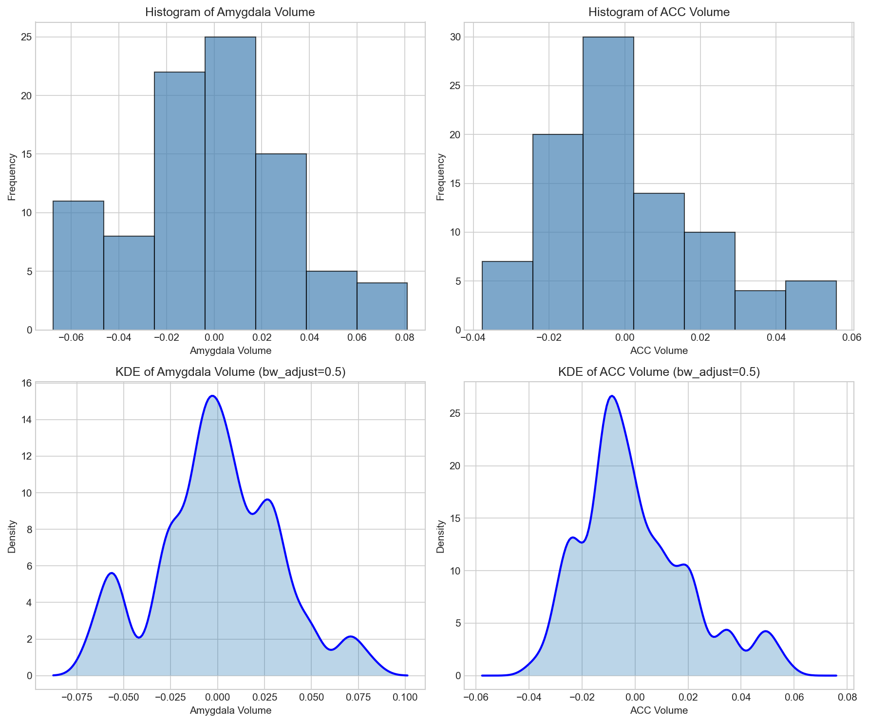 Top row: Histograms using Sturges’ rule for bin count. Bottom row: KDE with bandwidth factor 0.5. The KDE reveals a potential secondary mode in the amygdala distribution.
2D Analysis
Looking at both variables together:
from scipy.stats import gaussian_kde

X = data['amygdala'].values
Y = data['acc'].values

# Compute 2D KDE
kde = gaussian_kde(np.vstack([X, Y]), bw_method=0.3)

# Create grid for evaluation
x_grid, y_grid = np.mgrid[X.min():X.max():100j, Y.min():Y.max():100j]
positions = np.vstack([x_grid.ravel(), y_grid.ravel()])
z = kde(positions).reshape(x_grid.shape)

# Plot
plt.figure(figsize=(8, 6))
plt.contourf(x_grid, y_grid, z, levels=20, cmap='plasma')
plt.colorbar(label='Density')
plt.xlabel('Amygdala Volume')
plt.ylabel('ACC Volume')
plt.title('2D KDE of Brain Structure')
plt.show()
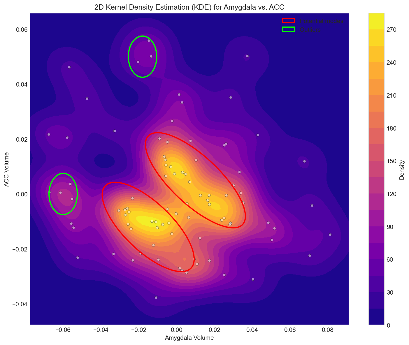 2D KDE of amygdala vs ACC volume. The contours suggest a primary mode with possible secondary structure. Red ellipses mark potential modes; green ellipses mark outliers.
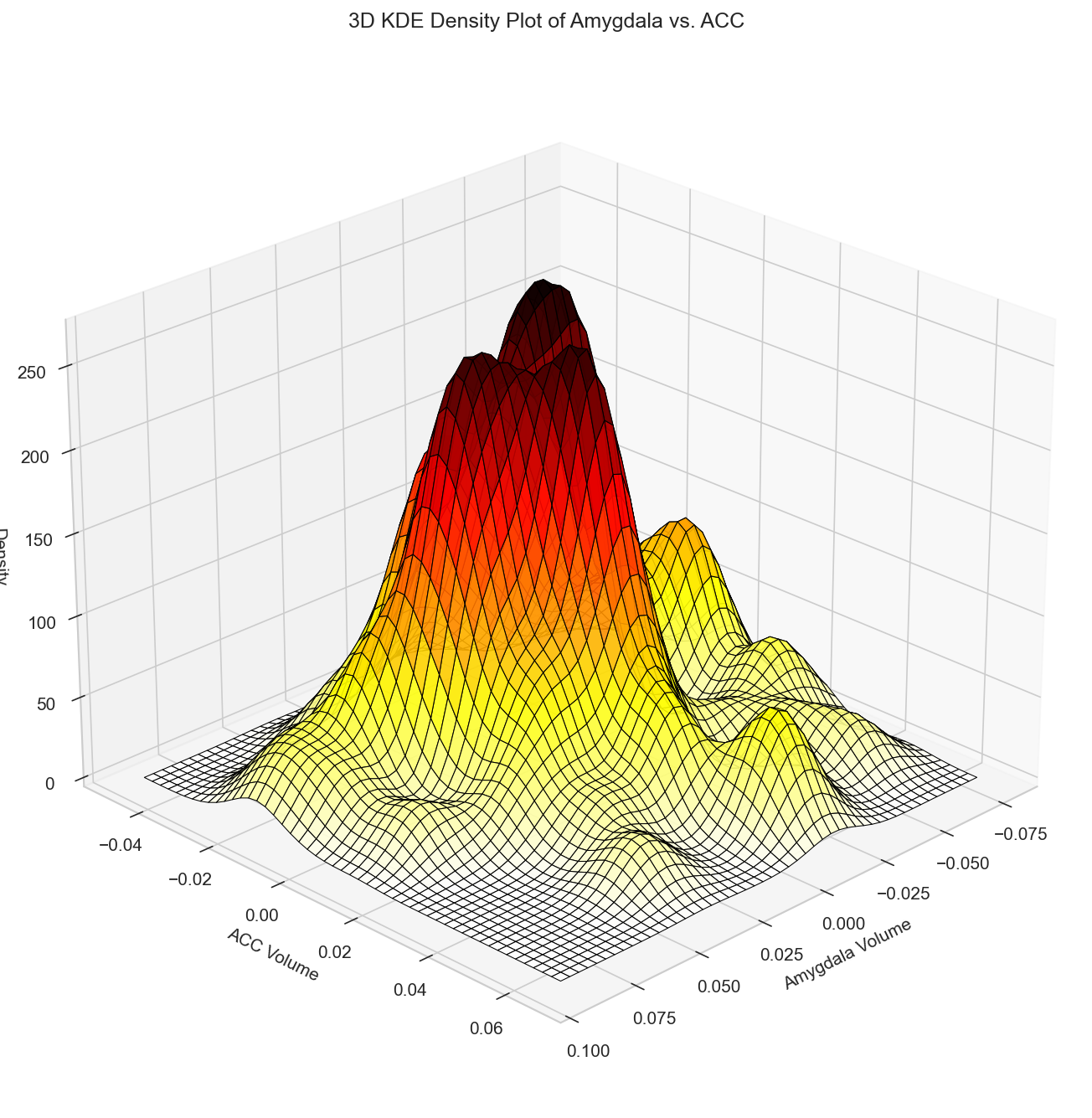 3D surface plot of the same density. The peaks and valleys are easier to see in this view.
Testing for Independence
Are amygdala and acc volumes independent?
from scipy.stats import pearsonr

corr, p_value = pearsonr(data['amygdala'], data['acc'])
print(f'Pearson correlation: {corr:.3f}')
print(f'p-value: {p_value:.3f}')
Results:
- Correlation: -0.13
- p-value: 0.23
The correlation is weak and not statistically significant. We can’t reject the null hypothesis that the variables are independent.
Conditional Distributions by Political Orientation
The more interesting question: do the distributions differ by political orientation?
# Plot conditional KDEs for each orientation
orientations = [2, 3, 4, 5]

plt.figure(figsize=(12, 6))
for c in orientations:
    subset = data[data['orientation'] == c]['amygdala']
    sns.kdeplot(subset, label=f'Orientation {c}', bw_adjust=0.6)

plt.xlabel('Amygdala Volume')
plt.ylabel('Density')
plt.title('Amygdala Volume by Political Orientation')
plt.legend()
plt.show()
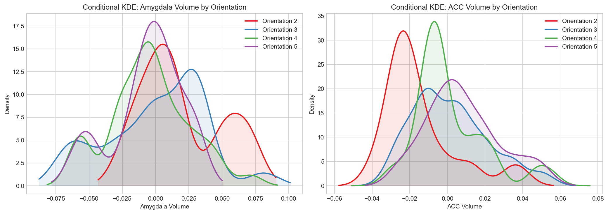 KDE of amygdala volume conditioned on political orientation. Orientation 2 (conservative) shows a distinct rightward shift compared to 4 and 5 (liberal).
| Orientation | Amygdala Mean | ACC Mean | Observations |
|---|---|---|---|
| 2 (Conservative) | 0.019 | -0.015 | Larger amygdala, smaller ACC |
| 3 (Lean Conservative) | 0.001 | 0.002 | Near average |
| 4 (Lean Liberal) | -0.005 | 0.001 | Smaller amygdala |
| 5 (Liberal) | -0.006 | 0.008 | Smaller amygdala, larger ACC |
The conditional 2D KDE plots show distinct patterns:
- Orientation 3 (neutral) has the widest spread in both dimensions
- Orientation 2 and 4 (leaning groups) show similar outlier patterns
- Orientation 5 (most liberal) has the narrowest distribution
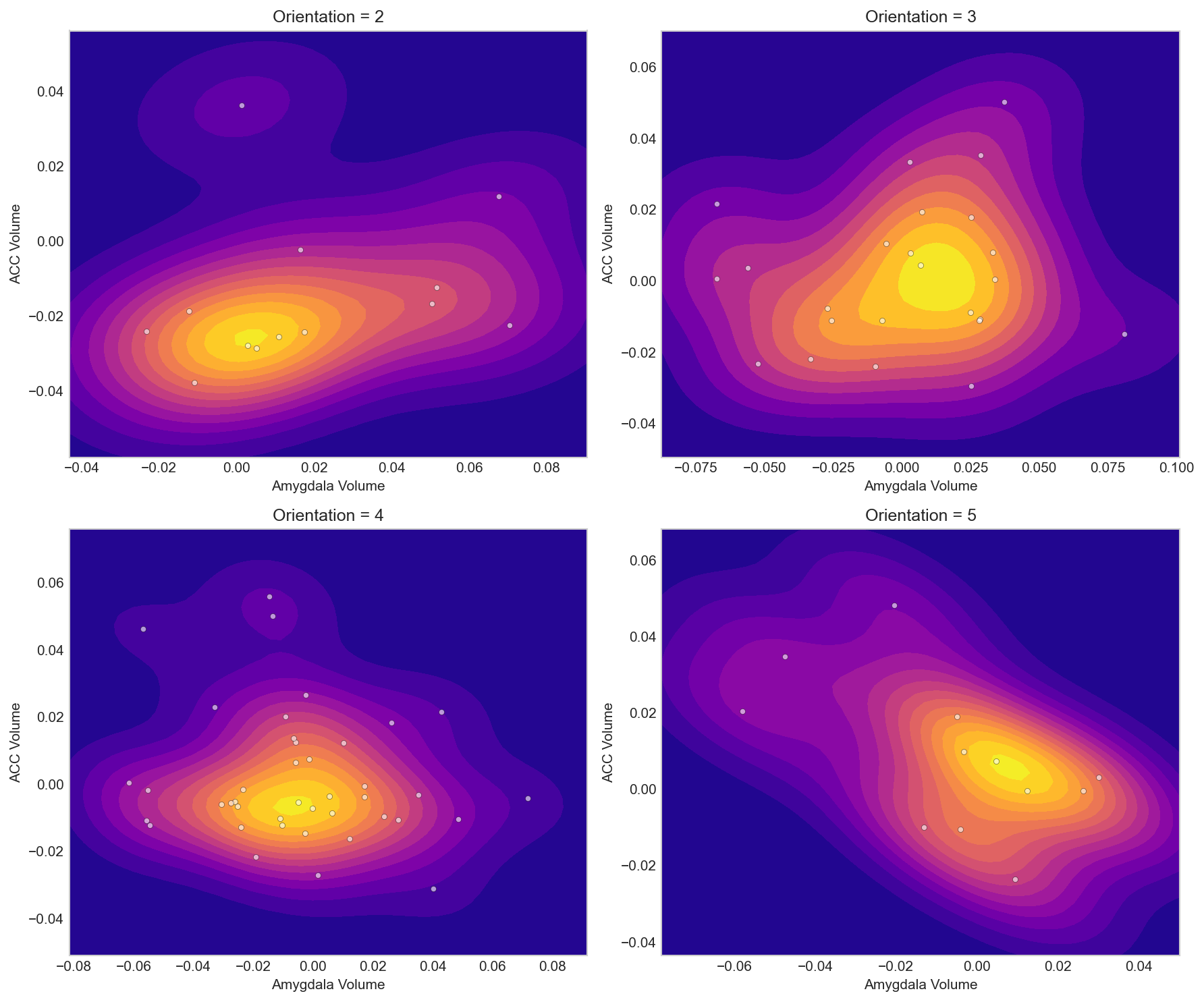 2D KDE of (amygdala, acc) for each political orientation. Orientation 3 (neutral) shows the widest spread, while more partisan orientations have tighter clusters.
Model Selection: How Many Components?
Using sklearn’s GaussianMixture to test whether the joint distribution is unimodal or multimodal:
from sklearn.mixture import GaussianMixture

X_joint = data[['amygdala', 'acc']].values

# Test different numbers of components
n_components_range = range(1, 7)
bics = []
aics = []

for n in n_components_range:
    gmm = GaussianMixture(n_components=n, random_state=0)
    gmm.fit(X_joint)
    bics.append(gmm.bic(X_joint))
    aics.append(gmm.aic(X_joint))

# Find optimal
best_bic = n_components_range[np.argmin(bics)]
best_aic = n_components_range[np.argmin(aics)]
print(f'Optimal components (BIC): {best_bic}')
print(f'Optimal components (AIC): {best_aic}')
Results:
- BIC suggests 1 component
- AIC suggests 3 components
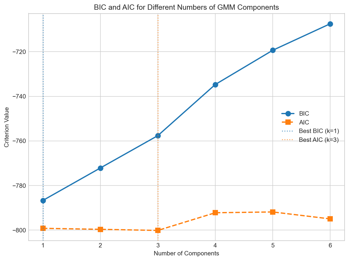 BIC and AIC for different numbers of GMM components. BIC (which penalizes complexity more) favors 1 component, while AIC suggests 3.
BIC penalizes complexity more heavily and is generally preferred for model selection. Despite what the KDE visually suggests, the statistical evidence doesn’t strongly support multiple components. This is a good reminder: visual patterns in small samples can be noise.
Application: Digit Classification with GMM
The Problem
We have 1,990 images of handwritten digits from MNIST: specifically, the digits 2 and 6. Can we classify them using GMM as a generative model, without ever telling the algorithm what the true labels are?
This is an example of unsupervised learning: we’ll fit a model to the data and see if it naturally discovers the two digit classes.
Why We Need PCA First
Each image is 28×28 = 784 pixels. That’s 784 dimensions. Why is this a problem for GMM?
-
Too many parameters: A full covariance matrix in 784D has $\frac{784 \times 785}{2} = 307,720$ parameters per component. With 2 components and only 1,990 data points, we’d be drastically overfitting.
-
Curse of dimensionality: In high dimensions, Gaussian densities become extremely peaked. Almost all points end up with near-zero density under any Gaussian.
-
Numerical instability: Covariance matrices become nearly singular (non-invertible) when dimensions exceed sample size.
The solution: Use PCA to reduce 784 dimensions to just 4. These 4 principal components capture the most important patterns of variation in the digit images.
What do the 4 principal components capture?
PCA finds the directions of maximum variance in the data. For digit images:
- PC1: Often captures overall brightness or stroke thickness
- PC2: May capture tilt/rotation of the digit
- PC3-4: Capture finer shape variations
The key insight: digits 2 and 6 differ systematically along these components. A 2 has a horizontal bottom and a curved top. A 6 has a loop at the bottom. These structural differences show up as different positions in PCA space.
Loading and Preprocessing
from scipy.io import loadmat
from sklearn.decomposition import PCA

# Load data
data_mat = loadmat('data.mat')
labels_mat = loadmat('label.mat')

# data.mat contains pixel values: shape (784, 1990)
# Each column is one 28x28 image, flattened
X = data_mat['data'].T  # Transpose to (1990, 784): one row per image
y = labels_mat['trueLabel'].flatten()  # True labels (we won't use these for training)

print(f'Data shape: {X.shape}')  # (1990, 784)
print(f'Unique labels: {np.unique(y)}')  # [2, 6]
print(f'Number of 2s: {np.sum(y == 2)}')  # ~1000
print(f'Number of 6s: {np.sum(y == 6)}')  # ~990

# Apply PCA: reduce from 784D to 4D
# This keeps the 4 directions that explain the most variance
pca = PCA(n_components=4)
X_pca = pca.fit_transform(X)

print(f'PCA shape: {X_pca.shape}')  # (1990, 4)
print(f'Variance explained: {pca.explained_variance_ratio_.sum():.1%}')  # ~40-50%
After PCA, each image is represented by just 4 numbers instead of 784. We lose some information, but we keep enough to distinguish 2s from 6s.
Fitting the GMM
Now we fit a 2-component GMM to the 4D PCA data. We set K=2 because we know there are two digit classes (though in practice, you might try different K values and use BIC to select).
# Run EM algorithm with K=2 components
# X_pca has shape (1990, 4): 1990 images, each represented by 4 PCA components
pi, mu, Sigma, gamma, log_likelihoods = em_gmm(X_pca, K=2, seed=1)

# Plot convergence to verify the algorithm worked
plt.figure(figsize=(8, 5))
plt.plot(log_likelihoods)
plt.xlabel('Iteration')
plt.ylabel('Log-Likelihood')
plt.title('EM Algorithm Convergence')
plt.show()

print(f'Final mixing weights: {pi}')
print(f'Converged in {len(log_likelihoods)} iterations')
What to expect:
- The log-likelihood should increase monotonically (EM guarantees this)
- It should plateau when the algorithm has converged
- The mixing weights should be roughly 50/50 since we have similar numbers of 2s and 6s
Results:
- $\pi_1 = 0.51$ (51% of data assigned to component 1)
- $\pi_2 = 0.49$ (49% of data assigned to component 2)
- Converged in ~18 iterations
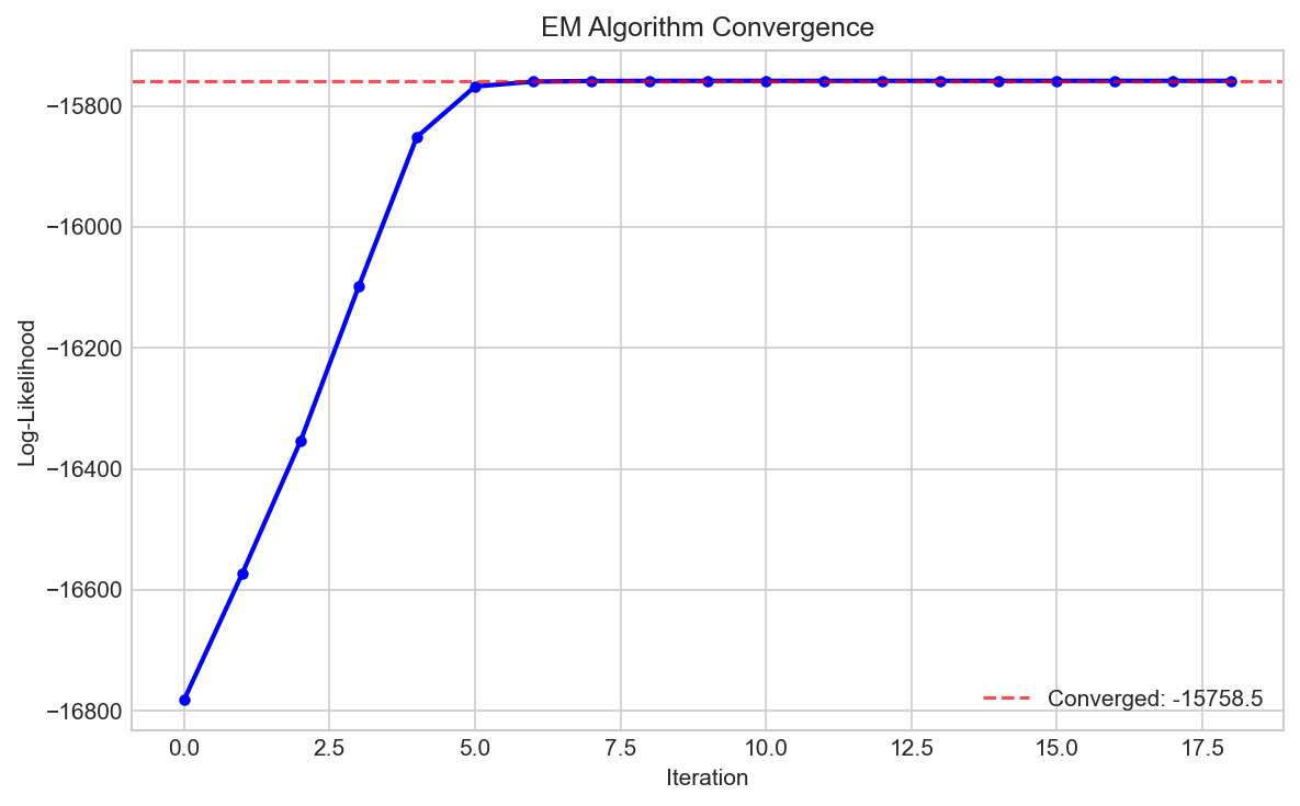 Log-likelihood increases monotonically and plateaus around iteration 15. The rapid convergence suggests the two digit classes are well-separated in PCA space.
What do the learned parameters mean?
Mixing weights π: These tell us what fraction of data belongs to each component. Getting ~50/50 makes sense because we have roughly equal numbers of 2s and 6s in the dataset.
Means μ (shape: 2×4): Each row is a 4D vector representing the "center" of one component in PCA space. These are abstract coordinates that we can map back to image space to visualize.
Covariances Σ (two 4×4 matrices): These capture how the data varies within each component. Different diagonal values mean different variances along different PCA directions. Off-diagonal values capture correlations between PCA components within each digit class.
Visualizing the Learned Means
Here’s the exciting part: can we see what the GMM learned? The mean $\mu_k$ of each component is a 4D vector (in PCA space). But we can map it back to the original 784D pixel space using pca.inverse_transform(), then reshape it to 28×28 to see it as an image.
# mu has shape (2, 4): two means, each with 4 PCA components
# inverse_transform maps from 4D PCA space back to 784D pixel space
mu_original = pca.inverse_transform(mu)  # Shape: (2, 784)

# Reshape each 784D vector into a 28x28 image and display
fig, axes = plt.subplots(1, 2, figsize=(8, 4))
for i in range(2):
    # Reshape from (784,) to (28, 28) for visualization
    mean_image = mu_original[i].reshape(28, 28)
    axes[i].imshow(mean_image, cmap='gray')
    axes[i].set_title(f'Mean Image of Component {i+1}')
    axes[i].axis('off')
plt.show()
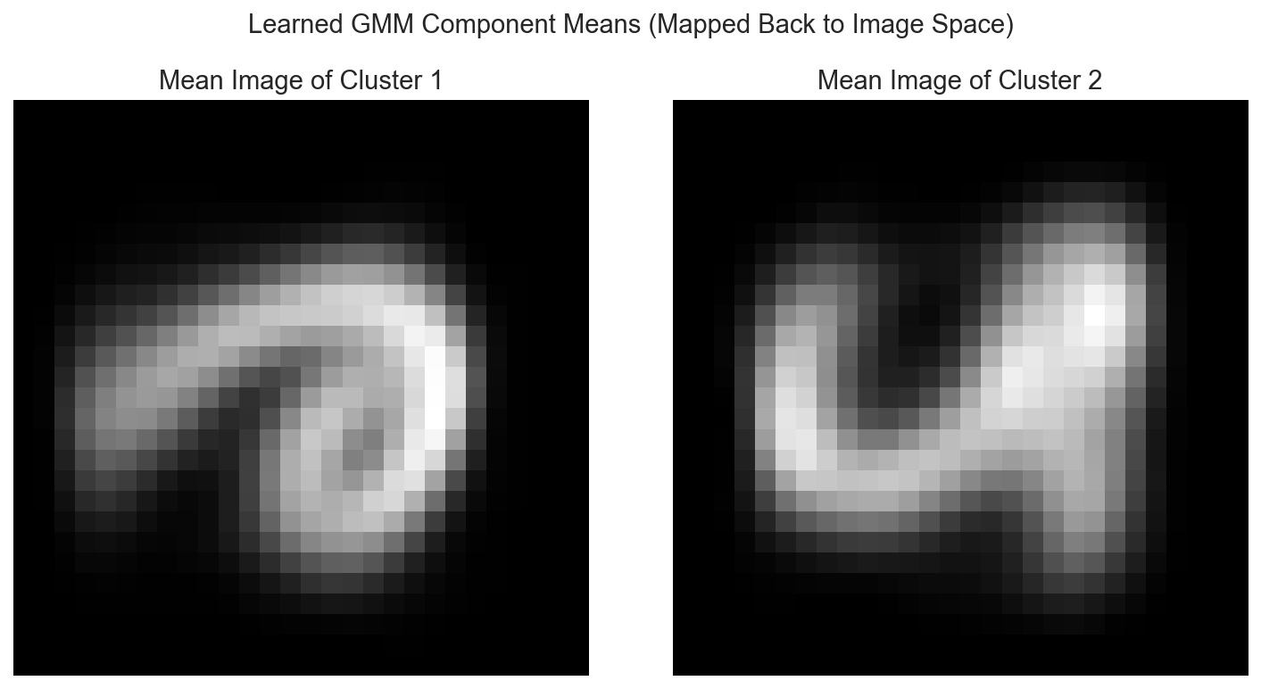 Mean images of the two GMM components, mapped back to 28×28 pixel space. One clearly resembles a “2”, the other resembles a “6”. The GMM discovered the digit structure without being told the labels.
This is remarkable: We never told the GMM that the data contains 2s and 6s. We just said “fit 2 components.” Yet the learned means clearly resemble the actual digits. The algorithm discovered the underlying structure purely from the data.
Why are the mean images slightly blurry?
Two reasons:
- PCA reconstruction loss: We compressed 784 dimensions to 4, then reconstructed. Some information is lost. The missing 780 dimensions contained fine details that can't be recovered.
- Averaging effect: The mean is an "average" of all digits assigned to that component. Handwritten 2s vary in slant, size, and style. Averaging them produces a blurry composite.
Despite the blur, the essential digit structure is clearly visible.
Covariance Structure
The GMM doesn’t just learn means. It also learns how data varies around each mean. This is captured in the 4×4 covariance matrices, one per component.
import seaborn as sns

# Sigma is a list of two 4x4 covariance matrices
fig, axes = plt.subplots(1, 2, figsize=(10, 4))
for i in range(2):
    sns.heatmap(Sigma[i], annot=True, fmt='.2f', ax=axes[i], cmap='RdBu_r',
                xticklabels=['PC1', 'PC2', 'PC3', 'PC4'],
                yticklabels=['PC1', 'PC2', 'PC3', 'PC4'])
    axes[i].set_title(f'Covariance Matrix of Component {i+1}')
plt.tight_layout()
plt.show()
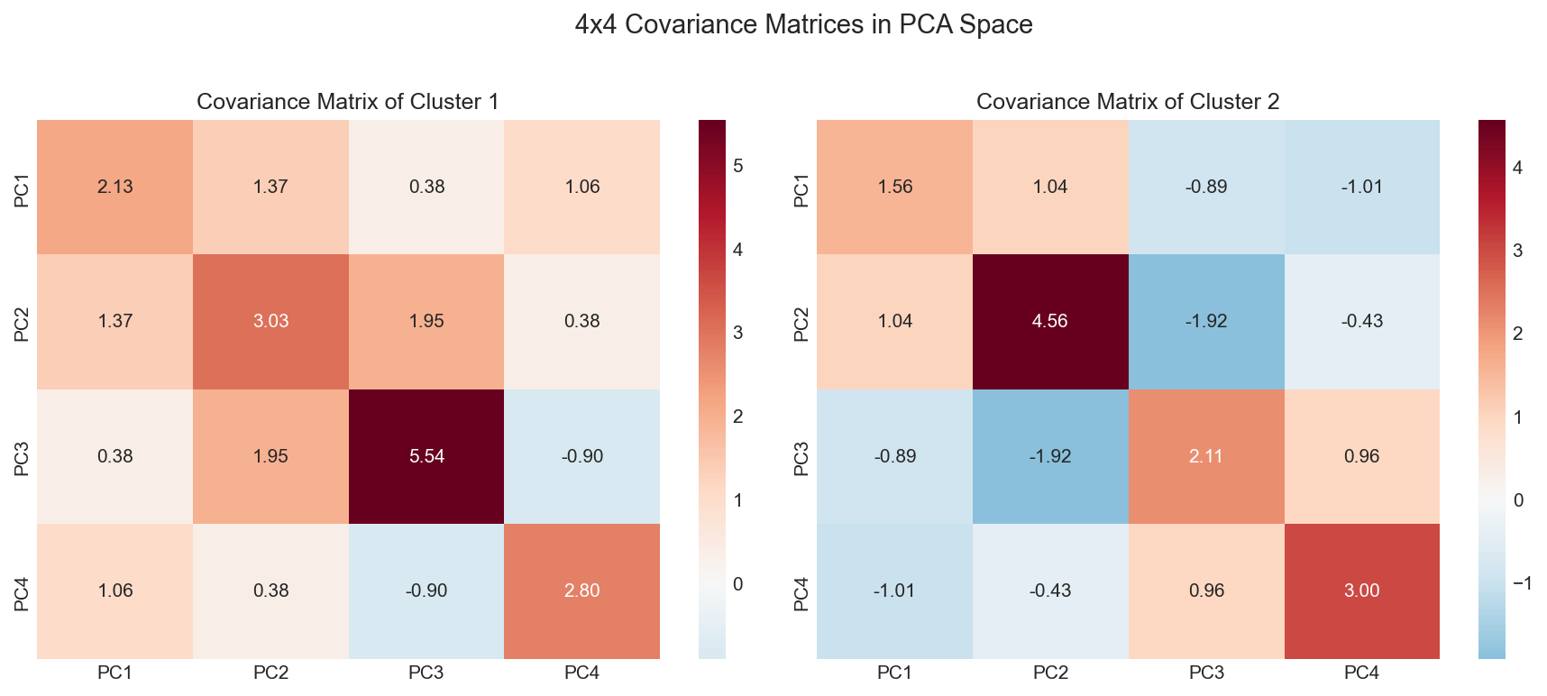 4×4 covariance matrices for each component in PCA space. The diagonal shows variance along each principal component. Off-diagonal shows correlations.
How to read these matrices
Diagonal entries (e.g., position [0,0]) show the variance along each principal component. Larger values mean more spread in that direction.
Off-diagonal entries (e.g., position [0,1]) show correlations between components. If positive, when PC1 increases, PC2 tends to increase too. If negative, they move in opposite directions.
Why the matrices differ: Digits 2 and 6 vary in different ways. For example:
- The curvature of a "2" might vary differently than the loop of a "6"
- The slant of a "2" might correlate with its height differently than for a "6"
By learning separate covariance matrices, the GMM captures these differences, leading to elliptical (not spherical) clusters that better fit the data.
Classification Results
Now we evaluate: how well did the GMM separate 2s from 6s? We assign each point to the component with higher responsibility, then compare to the true labels.
from sklearn.metrics import classification_report, confusion_matrix

# gamma has shape (1990, 2): responsibility of each point to each component
# For each point, pick the component with higher responsibility
predicted_clusters = np.argmax(gamma, axis=1)  # Shape: (1990,), values 0 or 1

# Problem: The GMM doesn't know which component is "2" vs "6"
# We need to figure out the mapping by looking at majority labels
cluster_0_labels = y[predicted_clusters == 0]  # True labels for points assigned to cluster 0
cluster_1_labels = y[predicted_clusters == 1]  # True labels for points assigned to cluster 1

# Determine mapping based on which digit is majority in each cluster
if np.sum(cluster_0_labels == 2) > np.sum(cluster_0_labels == 6):
    # Cluster 0 is mostly 2s, so map cluster 0 → digit 2
    cluster_to_digit = {0: 2, 1: 6}
else:
    # Cluster 0 is mostly 6s, so map cluster 0 → digit 6
    cluster_to_digit = {0: 6, 1: 2}

# Convert cluster assignments to digit predictions
predicted_digits = np.array([cluster_to_digit[c] for c in predicted_clusters])

# Evaluate against true labels
print('GMM Classification Results:')
print(confusion_matrix(y, predicted_digits))
print(classification_report(y, predicted_digits, target_names=['Digit 2', 'Digit 6']))
Understanding the confusion matrix
The confusion matrix shows:
| Predicted 2 | Predicted 6 | |
|---|---|---|
| Actual 2 | ~940 (correct) | ~60 (wrong) |
| Actual 6 | ~10 (wrong) | ~980 (correct) |
Most 2s are correctly identified as 2s, and most 6s as 6s. The ~70 errors are digits that look ambiguous or unusual.
Results comparison with K-Means:
| Metric | GMM | K-Means |
|---|---|---|
| Accuracy | 96% | 93% |
| Precision (Digit 2) | 0.99 | 0.93 |
| Recall (Digit 2) | 0.94 | 0.94 |
| Precision (Digit 6) | 0.93 | 0.93 |
| Recall (Digit 6) | 0.99 | 0.92 |
Why does GMM outperform K-Means?
-
Elliptical vs spherical clusters: K-Means assumes all clusters are spherical with equal variance. GMM learns a full covariance matrix, allowing elliptical clusters of different shapes and orientations. If 2s are spread out differently than 6s in PCA space, GMM can capture this.
-
Soft vs hard assignments: K-Means makes hard assignments (each point belongs to exactly one cluster). GMM gives soft probabilities. Points near the decision boundary get split responsibility, which often leads to better boundary estimation.
-
Probabilistic framework: GMM explicitly models the data-generating process. This tends to be more robust when the assumptions (Gaussian components) are approximately satisfied.
Summary
Histograms
- Simple and interpretable
- Sensitive to bin placement
- Discontinuous, can’t generate new samples
- Breaks down in high dimensions
Kernel Density Estimation
- Smooth, continuous density estimate
- Bandwidth is the key parameter (use Scott’s rule as starting point)
- Can sample from the estimated distribution
- Computationally expensive for large datasets
Gaussian Mixture Models
- Model data as a mixture of Gaussian components
- Learn parameters with EM algorithm
- Soft assignments: each point has probability of belonging to each component
- More flexible than K-Means (allows elliptical clusters)
EM Algorithm
- E-step: compute responsibilities using current parameters
- M-step: update parameters using responsibilities
- Guaranteed to increase log-likelihood each iteration
- Converges to local optimum (run multiple times)
General Principles
-
Bandwidth matters in KDE. Too small = overfitting, too large = oversmoothing. Start with Scott’s rule and adjust.
-
Use BIC/AIC for model selection. Don’t just pick the number of components that looks right visually.
-
GMM beats K-Means when clusters are elliptical. If your clusters are truly spherical, K-Means is simpler and faster.
-
EM finds local optima. Run multiple times with different initializations.
-
Visual patterns can be noise. Statistical tests often reveal that apparent structure isn’t significant, especially in small samples.
References
Kernel Density Estimation
- Silverman, B. W. (1986). Density Estimation for Statistics and Data Analysis. Chapman and Hall.
- Scott, D. W. (1992). Multivariate Density Estimation: Theory, Practice, and Visualization. Wiley.
Gaussian Mixture Models and EM
- Dempster, A. P., Laird, N. M., & Rubin, D. B. (1977). “Maximum Likelihood from Incomplete Data via the EM Algorithm.” Journal of the Royal Statistical Society: Series B, 39(1), 1-38.
- Bishop, C. M. (2006). Pattern Recognition and Machine Learning, Chapter 9. Springer.
Model Selection
- Schwarz, G. (1978). “Estimating the Dimension of a Model.” Annals of Statistics, 6(2), 461-464.
- Akaike, H. (1974). “A New Look at the Statistical Model Identification.” IEEE Transactions on Automatic Control, 19(6), 716-723.
Appendix: Complete Implementations
KDE Implementation
import numpy as np
from scipy.stats import gaussian_kde
import matplotlib.pyplot as plt

def kde_1d(data, bandwidth_factor=1.0):
    """1D Kernel Density Estimation."""
    kde = gaussian_kde(data)
    kde = gaussian_kde(data, bw_method=bandwidth_factor * kde.factor)
    return kde

def kde_2d(x, y, bandwidth_factor=1.0):
    """2D Kernel Density Estimation."""
    data = np.vstack([x, y])
    kde = gaussian_kde(data)
    kde = gaussian_kde(data, bw_method=bandwidth_factor * kde.factor)
    return kde

def plot_kde_2d(x, y, bandwidth_factor=0.5, grid_size=100):
    """Plot 2D KDE as contour."""
    kde = kde_2d(x, y, bandwidth_factor)

    x_grid, y_grid = np.mgrid[x.min():x.max():complex(grid_size),
                               y.min():y.max():complex(grid_size)]
    positions = np.vstack([x_grid.ravel(), y_grid.ravel()])
    z = kde(positions).reshape(x_grid.shape)

    plt.contourf(x_grid, y_grid, z, levels=20, cmap='plasma')
    plt.colorbar(label='Density')
    return kde
GMM with EM Implementation
import numpy as np
from scipy.stats import multivariate_normal

def em_gmm(X, K, max_iters=100, tol=1e-6, seed=None):
    """
    Fit GMM using Expectation-Maximization.

    Parameters:
    - X: data (n_samples, n_features)
    - K: number of components
    - max_iters: maximum iterations
    - tol: convergence tolerance
    - seed: random seed

    Returns:
    - pi: weights (K,)
    - mu: means (K, n_features)
    - Sigma: covariances list of (n_features, n_features)
    - gamma: responsibilities (n_samples, K)
    - log_likelihoods: convergence history
    """
    if seed is not None:
        np.random.seed(seed)

    n_samples, n_features = X.shape

    # Initialize
    mu = np.random.randn(K, n_features)
    Sigma = []
    for k in range(K):
        S = np.random.randn(n_features, n_features)
        Sigma.append(S @ S.T + np.eye(n_features))
    pi = np.ones(K) / K

    log_likelihoods = []

    for iteration in range(max_iters):
        # E-Step
        gamma = np.zeros((n_samples, K))
        for k in range(K):
            gamma[:, k] = pi[k] * multivariate_normal.pdf(X, mean=mu[k], cov=Sigma[k])
        gamma /= gamma.sum(axis=1, keepdims=True)

        # M-Step
        Nk = gamma.sum(axis=0)
        pi = Nk / n_samples

        for k in range(K):
            mu[k] = np.dot(gamma[:, k], X) / Nk[k]
            centered = X - mu[k]
            Sigma[k] = np.dot((gamma[:, k, None] * centered).T, centered) / Nk[k]

        # Log-likelihood
        ll = np.sum(np.log(np.sum([
            pi[k] * multivariate_normal.pdf(X, mean=mu[k], cov=Sigma[k])
            for k in range(K)
        ], axis=0)))
        log_likelihoods.append(ll)

        # Convergence check
        if iteration > 0 and abs(log_likelihoods[-1] - log_likelihoods[-2]) < tol:
            break

    return pi, mu, Sigma, gamma, log_likelihoods

def predict_gmm(X, pi, mu, Sigma):
    """Predict cluster assignments from fitted GMM."""
    K = len(pi)
    n_samples = X.shape[0]

    gamma = np.zeros((n_samples, K))
    for k in range(K):
        gamma[:, k] = pi[k] * multivariate_normal.pdf(X, mean=mu[k], cov=Sigma[k])
    gamma /= gamma.sum(axis=1, keepdims=True)

    return np.argmax(gamma, axis=1), gamma
Model Selection
from sklearn.mixture import GaussianMixture

def select_n_components(X, max_components=10):
    """Select optimal number of GMM components using BIC."""
    bics = []
    aics = []

    for n in range(1, max_components + 1):
        gmm = GaussianMixture(n_components=n, random_state=0)
        gmm.fit(X)
        bics.append(gmm.bic(X))
        aics.append(gmm.aic(X))

    best_bic = np.argmin(bics) + 1
    best_aic = np.argmin(aics) + 1

    return best_bic, best_aic, bics, aics
PS: This work was completed at Georgia Tech. The original submission files can be provided upon request to validate that this work is entirely my own.