Beyond Accuracy: Picking the Right Threshold When Costs Aren’t Equal

Most tutorials stop at accuracy. But what if a false negative costs you 10x more than a false positive?

---

Introduction

Logistic regression is one of those algorithms everyone learns but few people use correctly in production. The model outputs probabilities, not predictions. To get actual predictions, you need a threshold: if the probability exceeds 0.5, predict positive. Otherwise, predict negative.

But why 0.5? That number assumes false positives and false negatives are equally costly. They rarely are.

In this tutorial, we build a logistic regression model from scratch in R, understand the ROC curve, and then do what most tutorials skip: pick a threshold that minimizes actual business cost.

What we’ll cover:

• Building and evaluating a logistic regression model
• Understanding ROC curves and AUC in depth
• Finding the “optimal” threshold with Youden’s Index
• Going beyond Youden: cost-based threshold optimization
• When to use which approach

---

The Dataset

We’re using the German Credit dataset, a classic for credit risk modeling. Each row represents a loan applicant with features like credit history, loan duration, and employment status. The target tells us whether they defaulted (1) or not (0).

# Load the data
# Download from: https://archive.ics.uci.edu/dataset/144/statlog+german+credit+data
germancredit <- read.table("germancredit.txt", header = FALSE, sep = " ")
data <- germancredit

# Rename columns for clarity
# Suffix convention: _C = categorical, _I = integer, _B = binary
new_names <- c("existing_checking_C", "Duration_I", "Credit_hist_C", "Purpose_C",
               "Cred_Amt_I", "Savings_C", "Employed_Dur_C", "Rate_I", "Status_Sex_C",
               "Debt_C", "Residence_I", "Property_C", "Age_I", "Installment_Plans_C",
               "Housing_C", "Open_Credit_I", "Job_C", "Dependents_I", "Telephone_B",
               "International_Employee_B", "Target")
colnames(data) <- new_names

# Clean up
data <- unique(data)  # Remove duplicates

# Fix target: originally 1=good, 2=bad. Convert to 0/1
data$Target <- data$Target - 1

---

Preprocessing

Before modeling, we need to handle categorical variables. The key is one-hot encoding with the dummy variable trap in mind: drop one category per feature to avoid multicollinearity.

library(fastDummies)
library(caret)

# Identify categorical columns
cat_cols <- grep("_C$", colnames(data), value = TRUE)

# One-hot encode, dropping first dummy to prevent collinearity
data_encoded <- dummy_cols(data,
                           select_columns = cat_cols,
                           remove_first_dummy = TRUE,
                           remove_selected_columns = TRUE)

# Fix binary columns (stored as characters)
data_encoded$Telephone_B <- ifelse(data_encoded$Telephone_B == "A192", 1, 0)
data_encoded$International_Employee_B <- ifelse(data_encoded$International_Employee_B == "A201", 1, 0)

Why drop one dummy variable?

If you have 3 categories (Red, Green, Blue), you only need 2 dummy columns. Why? Because if Red=0 and Green=0, you know it must be Blue.

Keeping all 3 creates perfect multicollinearity: the third column is always determined by the first two. This breaks the math behind regression.

Color	Red	Green	Blue (redundant)
Red	1	0	0
Green	0	1	0
Blue	0	0	1

With just Red and Green columns, Blue is implied when both are 0.

---

Train-Test Split

library(caTools)

set.seed(123)  # For reproducibility
splitIndex <- sample.split(data_encoded$Target, SplitRatio = 0.7)

train_data <- data_encoded[splitIndex, ]
validation_data <- data_encoded[!splitIndex, ]

---

Building the Model

# Fit logistic regression
# family = binomial tells R we're doing logistic (not linear) regression
logistic_model <- glm(Target ~ ., data = train_data, family = binomial)

# Get predicted probabilities on validation set
predicted_probs <- predict(logistic_model, newdata = validation_data, type = "response")

The model outputs probabilities between 0 and 1. To make actual predictions, we need a threshold. The default is 0.5, but is that optimal?

---

Understanding the ROC Curve

The ROC (Receiver Operating Characteristic) curve is one of the most important tools for evaluating binary classifiers. It originated in World War II for analyzing radar signals (distinguishing enemy aircraft from noise), but it’s now standard in machine learning.

What the ROC Curve Shows

The ROC curve plots True Positive Rate (TPR) against False Positive Rate (FPR) at every possible threshold from 0 to 1.

True Positive Rate (Sensitivity/Recall):

\[TPR = \frac{TP}{TP + FN} = \frac{\text{Correctly identified positives}}{\text{All actual positives}}\]

False Positive Rate (1 - Specificity):

\[FPR = \frac{FP}{FP + TN} = \frac{\text{Incorrectly flagged negatives}}{\text{All actual negatives}}\]

Each point on the curve represents a different threshold. As you lower the threshold:

• You catch more true positives (TPR increases)
• But you also get more false positives (FPR increases)

The curve captures this tradeoff across all possible thresholds.

library(pROC)

roc_obj <- roc(validation_data$Target, predicted_probs)
plot(roc_obj, main = "ROC Curve", col = "#1c61b6", lwd = 2)
abline(a = 0, b = 1, lty = 2, col = "gray")  # Random classifier baseline

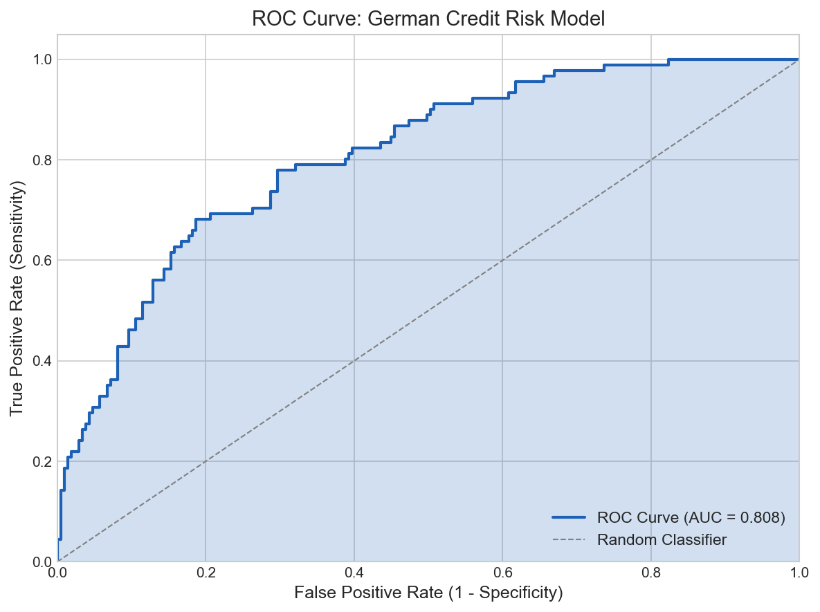The ROC curve for our credit risk model. The diagonal represents random guessing (AUC = 0.5). Our curve shows the model performs better than random.

How to Read the ROC Curve

The Axes:

• X-axis (False Positive Rate): The proportion of good customers incorrectly flagged as bad. Lower is better.
• Y-axis (True Positive Rate): The proportion of bad customers correctly identified. Higher is better.

Key Points on the Curve:

• Bottom-left corner (0,0): Threshold = 1.0. Predict everyone as negative. TPR = 0%, FPR = 0%.
• Top-right corner (1,1): Threshold = 0.0. Predict everyone as positive. TPR = 100%, FPR = 100%.
• Top-left corner (0,1): The perfect classifier. TPR = 100%, FPR = 0%.

The Diagonal Line: A random classifier (coin flip) produces the diagonal. Any model worth using should have a curve above this line.

See it with a tiny example

Imagine 4 predictions with these probabilities and true labels:

Sample	Probability	True Label
A	0.9	1 (bad)
B	0.7	1 (bad)
C	0.4	0 (good)
D	0.2	0 (good)

At threshold = 0.5:

• Predict 1 for A, B (both correct = 2 True Positives)
• Predict 0 for C, D (both correct = 2 True Negatives)
• TPR = 2/2 = 100%, FPR = 0/2 = 0%
• This is the point (0, 1) on the ROC curve. Perfect!

At threshold = 0.8:

• Only A gets predicted as 1
• B becomes a False Negative (we missed it)
• TPR = 1/2 = 50%, FPR = 0/2 = 0%
• This is the point (0, 0.5) on the ROC curve

At threshold = 0.3:

• A, B, C all get predicted as 1
• C becomes a False Positive
• TPR = 2/2 = 100%, FPR = 1/2 = 50%
• This is the point (0.5, 1) on the ROC curve

The ROC curve connects all these points as you sweep the threshold from 1 to 0.

Understanding AUC (Area Under the Curve)

The AUC summarizes the ROC curve in a single number between 0 and 1.

Interpretation:

\[AUC = P(\text{random positive ranked higher than random negative})\]

If you pick a random positive sample and a random negative sample, the AUC is the probability that your model assigns a higher score to the positive one.

AUC Value	Interpretation
0.5	Random guessing (useless model)
0.6-0.7	Poor discrimination
0.7-0.8	Acceptable discrimination
0.8-0.9	Excellent discrimination
0.9-1.0	Outstanding discrimination

Why AUC is Useful:

• It’s threshold-independent: You can compare models without choosing a threshold
• It’s scale-independent: Works the same whether probabilities range from 0.1-0.2 or 0.4-0.9
• It’s interpretable: The probabilistic interpretation makes sense to stakeholders

Limitations of AUC:

• It treats all thresholds equally, even ones you’d never use in practice
• It doesn’t account for class imbalance well
• It doesn’t reflect business costs

Calculating AUC manually

AUC can be computed using the trapezoidal rule:

1. Sort all predictions by threshold
2. At each threshold, compute (FPR, TPR)
3. Sum the trapezoid areas between consecutive points

Example with 4 samples:

Sorted by probability: A(0.9, y=1), B(0.7, y=1), C(0.4, y=0), D(0.2, y=0)

As we lower the threshold:

Threshold	TPR	FPR
1.0	0/2 = 0	0/2 = 0
0.9	1/2 = 0.5	0/2 = 0
0.7	2/2 = 1.0	0/2 = 0
0.4	2/2 = 1.0	1/2 = 0.5
0.2	2/2 = 1.0	2/2 = 1.0

The ROC curve goes: (0,0) → (0,0.5) → (0,1) → (0.5,1) → (1,1)

AUC = area under this curve = 1.0 (perfect separation in this example)

---

Finding the Optimal Threshold: Youden’s Index

If you want a balanced tradeoff between sensitivity and specificity, Youden’s Index helps. It finds the threshold that maximizes:

\[J = \text{Sensitivity} + \text{Specificity} - 1 = TPR - FPR\]

This is equivalent to finding the point on the ROC curve furthest from the diagonal.

# Extract all points on the ROC curve
full_coords <- coords(roc_obj, "all")
specificities <- full_coords$specificity
sensitivities <- full_coords$sensitivity
thresholds <- full_coords$threshold

# Calculate Youden's Index for each threshold
youden_indices <- sensitivities + specificities - 1

# Find the threshold with the highest Youden's Index
optimal_index <- which.max(youden_indices)
optimal_threshold <- thresholds[optimal_index]

print(paste("Optimal threshold (Youden):", round(optimal_threshold, 3)))

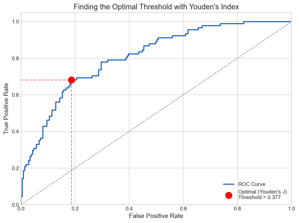The red point marks the optimal threshold according to Youden’s Index. This balances sensitivity and specificity equally.

Why Youden's Index works

Youden's J statistic measures the maximum vertical distance from the ROC curve to the diagonal line.

The intuition:

• At any threshold, Sensitivity + Specificity ranges from 0 to 2
• A random classifier has Sensitivity + Specificity = 1 (on the diagonal)
• Youden's J = (Sensitivity + Specificity) - 1 measures how much better than random
• The threshold that maximizes J gives the best balanced performance

Example calculation:

At threshold 0.4: Sensitivity = 0.85, Specificity = 0.70

• J = 0.85 + 0.70 - 1 = 0.55

At threshold 0.5: Sensitivity = 0.75, Specificity = 0.80

• J = 0.75 + 0.80 - 1 = 0.55

At threshold 0.6: Sensitivity = 0.60, Specificity = 0.85

• J = 0.60 + 0.85 - 1 = 0.45

In this example, thresholds 0.4 and 0.5 are equally optimal by Youden's criterion.

---

The Confusion Matrix

Using our optimal threshold, we can build the confusion matrix:

predicted_classes <- ifelse(predicted_probs > optimal_threshold, 1, 0)
confusion_matrix <- table(Predicted = predicted_classes, Actual = validation_data$Target)
print(confusion_matrix)

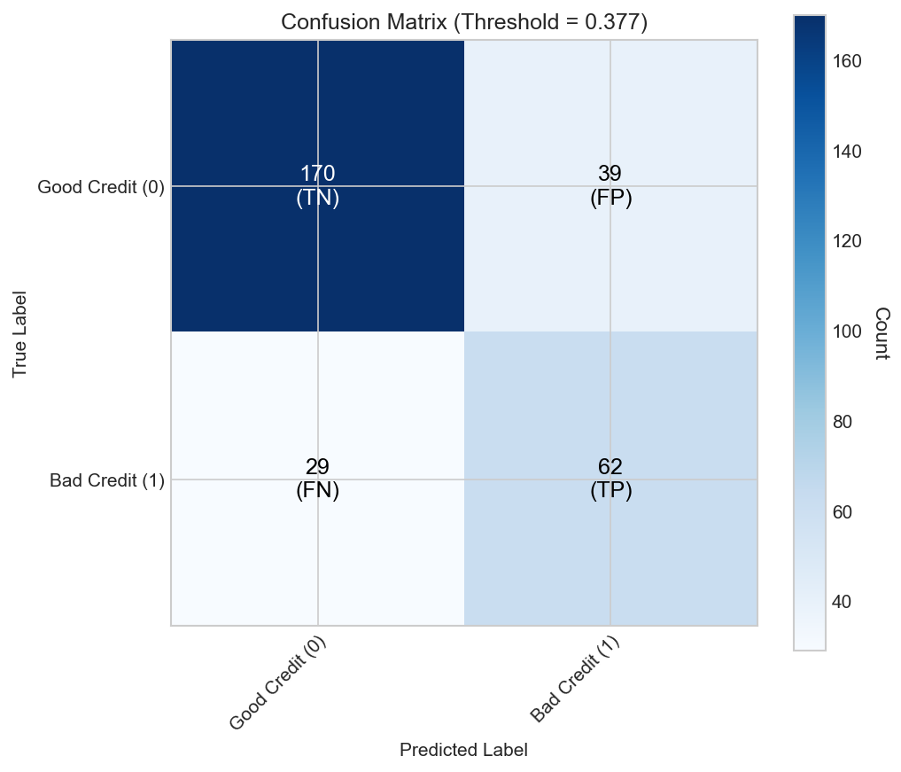The confusion matrix at the Youden-optimal threshold. TN = True Negative, FP = False Positive, FN = False Negative, TP = True Positive.

Reading the confusion matrix

	Actual 0 (Good)	Actual 1 (Bad)
Predicted 0	True Negative (TN)	False Negative (FN)
Predicted 1	False Positive (FP)	True Positive (TP)

From our model:

• TN: Good customers correctly approved
• FP: Good customers incorrectly denied (lost business)
• FN: Bad customers incorrectly approved (defaults!)
• TP: Bad customers correctly denied

Key metrics derived from the confusion matrix:

• Accuracy = (TN + TP) / (TN + FP + FN + TP)
• Precision = TP / (TP + FP)
• Recall (Sensitivity) = TP / (TP + FN)
• Specificity = TN / (TN + FP)
• F1 Score = 2 × (Precision × Recall) / (Precision + Recall)

---

When Accuracy Isn’t Enough

Here’s where it gets real. Youden’s Index assumes false positives and false negatives are equally bad. They rarely are.

Healthcare example:

• False Positive (healthy person diagnosed with disease): Unnecessary stress, tests, maybe invasive procedures
• False Negative (sick person cleared as healthy): Disease progresses, potentially fatal

In healthcare, you’d rather have more false positives than miss a single cancer case. You want high recall, even at the cost of precision.

Fraud detection example:

• False Positive (legitimate transaction blocked): Annoyed customer, maybe lost sale (5-50 dollars)
• False Negative (fraud goes through): Direct financial loss, chargebacks, fees (500-5000 dollars)

The costs depend on your business. A 10-dollar false positive and a 500-dollar false negative require very different thresholds.

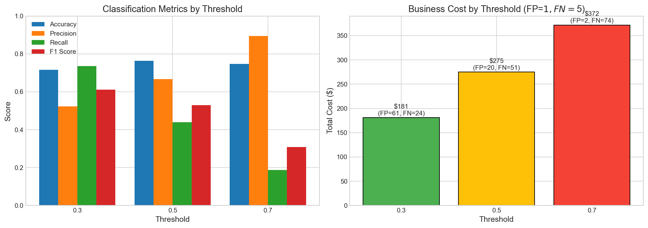Left: Classification metrics at different thresholds. Right: Business cost varies dramatically based on threshold choice.

---

Building a Cost-Based Optimizer

Let’s find the threshold that minimizes total business cost, not just maximizes some abstract metric.

# Define your costs
# Example: FP costs 1 (deny good customer), FN costs 5 (approve bad customer who defaults)
FP_Cost <- 1
FN_Cost <- 5

# Test every threshold from 0.1 to 0.9
threshold_seq <- seq(0.1, 0.9, 0.01)

# Store results
costs_df <- data.frame(threshold = numeric(), cost = numeric(),
                       FP = numeric(), FN = numeric())

for (threshold in threshold_seq) {
  # Classify at this threshold
  predicted_classes <- ifelse(predicted_probs > threshold, 1, 0)

  # Build confusion matrix
  cm <- table(Predicted = predicted_classes, Actual = validation_data$Target)

  # Handle edge cases
  if (nrow(cm) != 2 || ncol(cm) != 2) next

  # Extract values
  FP <- cm[2, 1]  # Predicted 1, Actual 0
  FN <- cm[1, 2]  # Predicted 0, Actual 1

  # Calculate total cost
  total_cost <- FP * FP_Cost + FN * FN_Cost

  costs_df <- rbind(costs_df,
                    data.frame(threshold = threshold, cost = total_cost,
                               FP = FP, FN = FN))
}

# Find minimum cost threshold
optimal_idx <- which.min(costs_df$cost)
cost_optimal_threshold <- costs_df$threshold[optimal_idx]

print(paste("Cost-optimal threshold:", cost_optimal_threshold))
print(paste("Minimum cost:", costs_df$cost[optimal_idx]))

What happens if you change the costs? If FN_Cost is much higher than FP_Cost (like in healthcare), the optimal threshold shifts lower. The model becomes more aggressive about predicting positives to avoid missing any. If FP_Cost is higher (like in spam filtering where false positives annoy users), the threshold shifts higher.

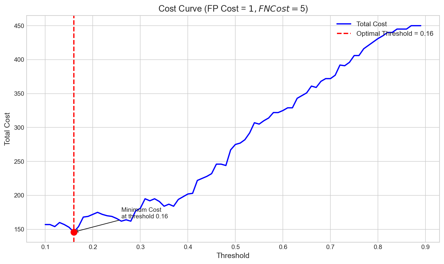Total cost as a function of threshold. The red line marks the cost-optimal threshold, which may differ from the Youden-optimal threshold.

---

How Cost Structure Changes the Optimal Threshold

Different business problems have different cost structures:

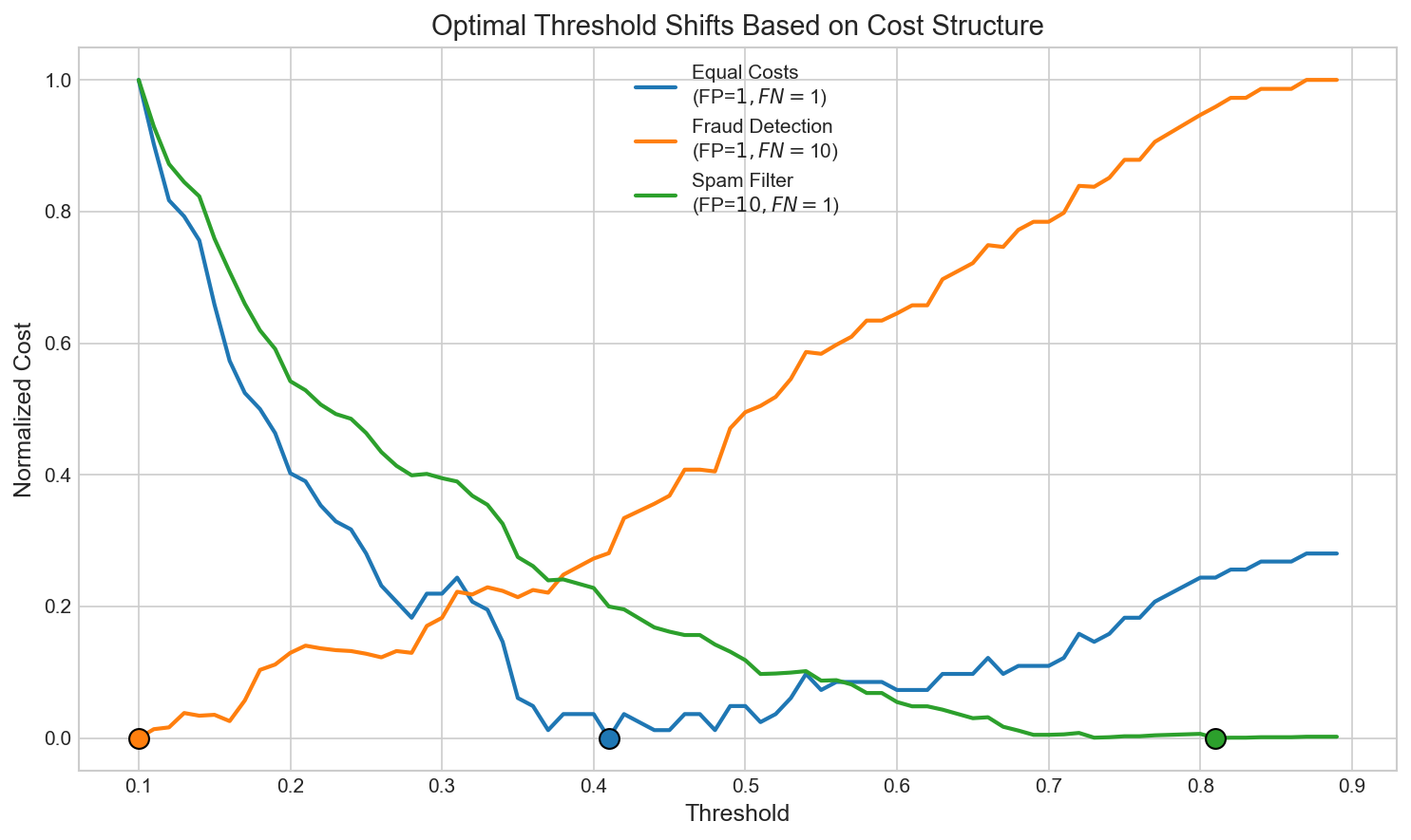The optimal threshold shifts based on the cost structure. Fraud detection (high FN cost) pushes the threshold lower. Spam filtering (high FP cost) pushes it higher.

Scenario	FP Cost	FN Cost	Optimal Threshold
Equal costs	1	1	~0.50 (balanced)
Fraud detection	1	10	Lower (~0.30)
Spam filter	10	1	Higher (~0.70)
Medical screening	1	100	Very low (~0.10)

---

When Would You Use This?

Use Youden’s Index when:

• You don’t have clear cost information
• False positives and false negatives are roughly equally bad
• You want a quick, defensible baseline

Use cost-based optimization when:

• You have actual dollar costs for each error type
• The costs are meaningfully different (at least 2-3x)
• You’re deploying to production and care about business outcomes

Neither approach when:

• Your model has terrible AUC (< 0.6). Fix the model first.
• The costs change frequently. Build a system that recalculates thresholds.
• You have massive class imbalance. Consider sampling techniques first.

---

Summary

1. Logistic regression outputs probabilities, not classes. You need a threshold to convert them.

2. The ROC curve shows all possible thresholds and their tradeoffs between true positive rate and false positive rate.

3. AUC summarizes model performance in a single number: the probability that a random positive is ranked higher than a random negative.

4. Youden’s Index finds a balanced threshold, but assumes equal costs for both types of errors.

5. Cost-based optimization finds the threshold that minimizes actual business cost. This is what you should use in production.

6. Always define your costs first. Talk to stakeholders. What does a false positive cost? A false negative? The math is easy once you know the numbers.

---

Appendix: Complete R Script

Full Implementation

# ============================================
# Logistic Regression with Cost-Based Thresholds
# ============================================

# Load packages
library(caTools)
library(fastDummies)
library(caret)
library(pROC)

# ----- Data Loading -----
germancredit <- read.table("germancredit.txt", header = FALSE, sep = " ")
data <- germancredit

new_names <- c("existing_checking_C", "Duration_I", "Credit_hist_C", "Purpose_C",
               "Cred_Amt_I", "Savings_C", "Employed_Dur_C", "Rate_I", "Status_Sex_C",
               "Debt_C", "Residence_I", "Property_C", "Age_I", "Installment_Plans_C",
               "Housing_C", "Open_Credit_I", "Job_C", "Dependents_I", "Telephone_B",
               "International_Employee_B", "Target")
colnames(data) <- new_names
data <- unique(data)
data$Target <- data$Target - 1

# ----- Preprocessing -----
cat_cols <- grep("_C$", colnames(data), value = TRUE)
data_encoded <- dummy_cols(data, select_columns = cat_cols,
                           remove_first_dummy = TRUE, remove_selected_columns = TRUE)
data_encoded$Telephone_B <- ifelse(data_encoded$Telephone_B == "A192", 1, 0)
data_encoded$International_Employee_B <- ifelse(data_encoded$International_Employee_B == "A201", 1, 0)

# ----- Train/Test Split -----
set.seed(123)
splitIndex <- sample.split(data_encoded$Target, SplitRatio = 0.7)
train_data <- data_encoded[splitIndex, ]
validation_data <- data_encoded[!splitIndex, ]

# ----- Model Training -----
logistic_model <- glm(Target ~ ., data = train_data, family = binomial)
predicted_probs <- predict(logistic_model, newdata = validation_data, type = "response")

# ----- ROC Curve -----
roc_obj <- roc(validation_data$Target, predicted_probs)
print(paste("AUC:", round(auc(roc_obj), 3)))

# ----- Youden's Index -----
full_coords <- coords(roc_obj, "all")
youden_indices <- full_coords$sensitivity + full_coords$specificity - 1
youden_threshold <- full_coords$threshold[which.max(youden_indices)]
print(paste("Youden optimal threshold:", round(youden_threshold, 3)))

# ----- Cost-Based Optimization -----
FP_Cost <- 1
FN_Cost <- 5

costs_df <- data.frame(threshold = numeric(), cost = numeric())

for (threshold in seq(0.1, 0.9, 0.01)) {
  predicted_classes <- ifelse(predicted_probs > threshold, 1, 0)
  cm <- table(Predicted = predicted_classes, Actual = validation_data$Target)

  if (nrow(cm) == 2 && ncol(cm) == 2) {
    FP <- cm[2, 1]
    FN <- cm[1, 2]
    cost <- FP * FP_Cost + FN * FN_Cost
    costs_df <- rbind(costs_df, data.frame(threshold = threshold, cost = cost))
  }
}

cost_optimal <- costs_df$threshold[which.min(costs_df$cost)]
print(paste("Cost-optimal threshold:", cost_optimal))

# ----- Final Evaluation -----
final_predictions <- ifelse(predicted_probs > cost_optimal, 1, 0)
final_cm <- table(Predicted = final_predictions, Actual = validation_data$Target)
print("Final Confusion Matrix:")
print(final_cm)