Clustering Algorithms From Scratch
You have 10,000 data points. How do you find natural groupings without any labels?
Introduction
Clustering is one of those things that sounds simple until you try to implement it. “Group similar things together.” Easy, right? But what does “similar” mean? How many groups should there be? What if your data has weird shapes?
In this tutorial, we build two clustering algorithms from scratch:
- K-Means: The classic. Fast, interpretable, but assumes spherical clusters.
- Spectral Clustering: Handles complex shapes by transforming the problem into a graph.
We will apply K-Means to image compression (reducing millions of colors to just a few) and Spectral Clustering to network analysis (finding communities in a graph of political blogs).
All code is in NumPy. Obviously in practice you should pull Sklearn and do this in minutes, but this is a basic implementation of the algorithms underneath the packages.
Just want the code? Skip to the Appendix for copy-paste ready implementations.
Part 1: K-Means Clustering
Problem Statement
Given $n$ data points ${x_1, x_2, \ldots, x_n}$ in $\mathbb{R}^d$, we want to partition them into $k$ clusters such that points within each cluster are as similar as possible.
The objective is to minimize the within-cluster sum of squares:
\[J = \sum_{j=1}^{k} \sum_{x_i \in C_j} \|x_i - \mu_j\|^2\]Where:
- $C_j$ is the set of points assigned to cluster $j$
- $\mu_j$ is the centroid (mean) of cluster $j$
- $|x_i - \mu_j|^2$ is the squared Euclidean distance
How the Algorithm Works
K-Means uses an iterative refinement approach:
- Initialize: Randomly select $k$ data points as initial centroids
- Assign: For each point, find the nearest centroid and assign the point to that cluster
- Update: Recalculate each centroid as the mean of all points assigned to it
- Repeat: Go back to step 2 until centroids stop moving (or move very little)
Why does this work? Each step either decreases the objective $J$ or leaves it unchanged. Assigning points to their nearest centroid minimizes distances given fixed centroids. Updating centroids to cluster means minimizes distances given fixed assignments. Since $J$ is bounded below by zero and decreases monotonically, the algorithm must converge.
See it with a tiny example
6 points in 2D, finding k=2 clusters:
| Point | X | Y |
|---|---|---|
| A | 1 | 1 |
| B | 2 | 1 |
| C | 1 | 2 |
| D | 8 | 8 |
| E | 9 | 8 |
| F | 8 | 9 |
Iteration 1:
- Random centroids: C1=(1,1), C2=(9,8)
- Assign: A,B,C → C1 (closer), D,E,F → C2
- Update: C1 = mean(A,B,C) = (1.33, 1.33), C2 = mean(D,E,F) = (8.33, 8.33)
Iteration 2:
- Assign: same assignments (centroids barely moved)
- Update: same centroids
- Converged!
Final clusters: {A,B,C} and {D,E,F}
Implementation
Let’s build it piece by piece.
Step 1: Cluster Assignment
def assign_clusters(data, centroids, norm=2):
    """
    Assign each data point to its nearest centroid.

    Parameters:
    - data: array of shape (n_samples, n_features)
    - centroids: array of shape (k_clusters, n_features)
    - norm: which distance metric (2 = Euclidean, 1 = Manhattan)

    Returns:
    - labels: array of shape (n_samples,) with cluster assignments 0 to k-1
    """
    # Calculate distance from each point to each centroid
    # data[:, np.newaxis] adds a dimension so we can broadcast against all k centroids
    # Original shape: (n_samples, n_features)
    # After newaxis: (n_samples, 1, n_features)
    # Centroids shape: (k_clusters, n_features)
    # Result of subtraction: (n_samples, k_clusters, n_features)
    # After norm: (n_samples, k_clusters)
    distances = np.linalg.norm( # there is another version of this function that I wasn't able to use.
        data[:, np.newaxis] - centroids,
        axis=2,
        ord=norm
    )

    # For each point, find which centroid is closest
    # argmin returns the INDEX of the minimum value
    return np.argmin(distances, axis=1)
What happens if you change this? Setting norm=1 switches to Manhattan distance (sum of absolute differences). Manhattan distance is less sensitive to outliers and works better when your features have different scales or when you care about axis-aligned distances.
Step 2: Centroid Update
def update_centroids(data, labels, k):
    """
    Compute new centroids as the mean of assigned points.

    Parameters:
    - data: array of shape (n_samples, n_features)
    - labels: array of shape (n_samples,) with cluster assignments
    - k: number of clusters

    Returns:
    - new_centroids: array of shape (k_clusters, n_features)
    """
    n_features = data.shape[1]
    centroids = np.zeros((k, n_features))

    for j in range(k):
        # Find all points belonging to cluster j
        cluster_points = data[labels == j]

        if len(cluster_points) > 0:
            # Centroid is the mean of all points in the cluster
            centroids[j] = cluster_points.mean(axis=0)
        else:
            # Empty cluster! Reinitialize to a random data point
            centroids[j] = data[np.random.randint(len(data))]

    return centroids
What happens if you change this? Empty clusters are a real problem for a manual implementation like this. If a centroid drifts away from all data points, it gets no assignments and becomes useless. The code above handles this by reinitializing to a random point. Another approach is to reinitialize to the point furthest from its assigned centroid, which spreads centroids more evenly.
Step 3: Convergence Check
def has_converged(old_centroids, new_centroids, tolerance=1e-4):
    """
    Check if centroids have stopped moving.

    We measure the total movement of all centroids and compare to a tolerance.
    """
    # Sum of squared distances between old and new centroid positions
    shift = np.sum((old_centroids - new_centroids) ** 2)
    return shift < tolerance
What happens if you change this? A larger tolerance (like 0.1) makes the algorithm stop earlier, potentially before centroids have fully settled. A smaller tolerance (like 0.0001) gives more precision but takes more iterations. For image compression, you often do not need high precision since visual differences are imperceptible.
Putting It Together
def kmeans(data, k, norm=2, max_iters=100, tolerance=1e-4, seed=None):
    """
    Full K-Means implementation.

    Parameters:
    - data: array of shape (n_samples, n_features)
    - k: number of clusters
    - norm: distance metric (2 = Euclidean, 1 = Manhattan)
    - max_iters: maximum iterations before stopping
    - tolerance: convergence threshold
    - seed: random seed for reproducibility

    Returns:
    - labels: cluster assignments
    - centroids: final centroid positions
    - iterations: number of iterations until convergence
    """
    if seed is not None:
        np.random.seed(seed)

    n_samples = data.shape[0]

    # Initialize: randomly select k data points as starting centroids
    # This is called "Forgy initialization"
    random_indices = np.random.choice(n_samples, size=k, replace=False)
    centroids = data[random_indices].copy()

    for iteration in range(max_iters):
        # Step 1: Assign each point to nearest centroid
        labels = assign_clusters(data, centroids, norm)

        # Step 2: Update centroids to cluster means
        new_centroids = update_centroids(data, labels, k)

        # Step 3: Check for convergence
        if has_converged(centroids, new_centroids, tolerance):
            return labels, new_centroids, iteration + 1

        centroids = new_centroids

    # Did not converge within max_iters
    return labels, centroids, max_iters
Handling Initialization Sensitivity
K-Means has a dirty secret: the final result depends heavily on where you start. Bad initialization can lead to poor local minima.
def kmeans_best_of_n(data, k, n_runs=10, **kwargs):
    """
    Run K-Means multiple times and keep the best result.

    "Best" means lowest within-cluster sum of squares (WCSS).
    """
    best_labels = None
    best_centroids = None
    best_wcss = float('inf')

    for run in range(n_runs):
        labels, centroids, _ = kmeans(data, k, seed=run, **kwargs)

        # Calculate within-cluster sum of squares
        wcss = 0
        for j in range(k):
            cluster_points = data[labels == j]
            if len(cluster_points) > 0:
                wcss += np.sum((cluster_points - centroids[j]) ** 2)

        if wcss < best_wcss:
            best_wcss = wcss
            best_labels = labels
            best_centroids = centroids

    return best_labels, best_centroids, best_wcss
What happens if you change this? More runs increase your chances of finding a good solution but take longer. For most applications, 10 runs is sufficient. If you run this multiple times with different seeds, you will notice the WCSS varies. The variance decreases as you increase n_runs.
Application: Image Compression
Problem Statement
A color image is just a matrix of RGB values. Each pixel has three numbers (red, green, blue), each ranging from 0 to 255. A 400x225 image has 90,000 pixels, and if each pixel can be any of 16.7 million colors ($256^3$), that is a lot of data.
What if we limited the image to just $k$ colors? We would lose some detail, but the file size shrinks dramatically. This is lossy compression.
The approach:
- Treat each pixel as a 3D point (R, G, B)
- Run K-Means to find $k$ cluster centroids
- Replace each pixel with its nearest centroid color
Results
| k (colors) | Converged | Iterations | Visual Quality |
|---|---|---|---|
| 3 | Yes | 14 | Posterized, obvious color banding |
| 6 | Yes | 19 | Better gradients, still simplified |
| 12 | Yes | 23 | Good for graphics, slight loss on photos |
| 24 | Yes | 31 | Harder to distinguish from original |
 Original image with millions of possible colors
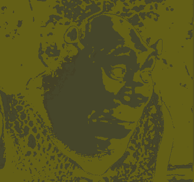 k=3: Only three colors. Dramatic posterization effect.
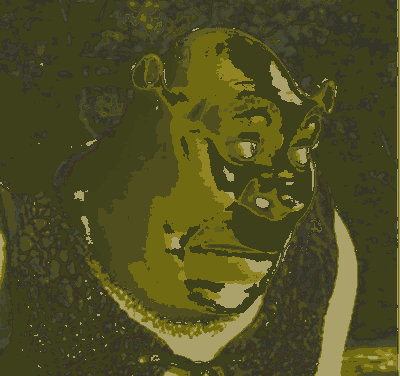 k=12: Still a bit shaky on the details.
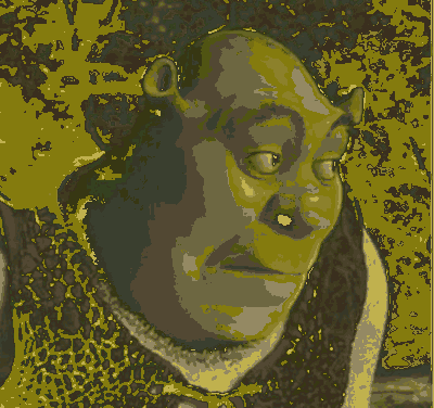 k=24: The colors start to resemble the original.
Honestly, there is probably a way to make good pixel-art out of this.
Compression Code
def compress_image(image_path, k, norm=2):
    """
    Compress an image to k colors using K-Means.

    Parameters:
    - image_path: path to the input image
    - k: number of colors in compressed image
    - norm: distance metric for K-Means

    Returns:
    - compressed: the compressed image array
    - centroids: the k colors used
    """
    # Load image and get dimensions
    img = plt.imread(image_path)
    height, width, channels = img.shape

    # Reshape from (H, W, 3) to (H*W, 3)
    # Each row is now one pixel with R, G, B values
    pixels = img.reshape(-1, 3)

    # Convert to float if needed (some images are 0-255 integers)
    if pixels.max() > 1:
        pixels = pixels / 255.0

    # Run K-Means to find k representative colors
    labels, centroids, iterations = kmeans(pixels, k, norm=norm)

    # Replace each pixel with its centroid color
    compressed_pixels = centroids[labels]

    # Reshape back to image dimensions
    compressed = compressed_pixels.reshape(height, width, channels)

    return compressed, centroids
Euclidean vs Manhattan Distance
Does the distance metric matter for image compression?
| Metric | k=12 WCSS | Visual Difference |
|---|---|---|
| Euclidean (L2) | 0.0142 | Smooth gradients |
| Manhattan (L1) | 0.0156 | Slightly more saturated colors |
The difference is subtle. Euclidean tends to produce colors that are perceptually “average,” while Manhattan can produce colors that are slightly more vivid because it weights each RGB channel equally rather than penalizing large deviations in any single channel.
Part 2: Spectral Clustering
The Problem with K-Means
K-Means assumes clusters are spherical. It draws straight lines between cluster centers. What if your data looks like two interlocking spirals? Or two concentric circles? K-Means fails badly.
Spectral Clustering takes a different approach: instead of clustering points directly in their original space, we first transform them into a space where clusters become separable.
The Core Idea
Plain English: We build a graph where similar points are connected. Then we find a way to “cut” the graph into pieces such that we cut as few edges as possible.
Why this helps: If two points are similar, they are connected. If two clusters exist, there should be fewer connections between clusters than within them. Finding a good cut means finding the natural cluster boundaries.
The trick: Instead of literally finding cuts (which is NP-hard), we use the eigenvectors of a special matrix called the Graph Laplacian. The eigenvectors magically encode cluster membership.
The Graph Laplacian
Plain English: The Laplacian is a matrix that captures how “different” each node is from its neighbors.
Intuition: Imagine spreading heat through a network. Heat flows easily between connected nodes. The Laplacian describes this diffusion process. Clusters act like insulated regions where heat stays trapped.
The formula:
Given a graph with $n$ nodes:
-
Adjacency matrix $A$: An $n \times n$ matrix where $A_{ij} = 1$ if node $i$ connects to node $j$, and 0 otherwise.
-
Degree matrix $D$: A diagonal matrix where $D_{ii}$ equals the number of connections for node $i$.
-
Graph Laplacian: $L = D - A$
See it with a tiny example
Consider 4 nodes with this connection pattern:
1 --- 2
|     |
3 --- 4
Adjacency matrix A (who connects to whom):
| 1 | 2 | 3 | 4 | |
|---|---|---|---|---|
| 1 | 0 | 1 | 1 | 0 |
| 2 | 1 | 0 | 0 | 1 |
| 3 | 1 | 0 | 0 | 1 |
| 4 | 0 | 1 | 1 | 0 |
Degree matrix D (count of connections per node):
| 1 | 2 | 3 | 4 | |
|---|---|---|---|---|
| 1 | 2 | 0 | 0 | 0 |
| 2 | 0 | 2 | 0 | 0 |
| 3 | 0 | 0 | 2 | 0 |
| 4 | 0 | 0 | 0 | 2 |
Laplacian L = D - A:
| 1 | 2 | 3 | 4 | |
|---|---|---|---|---|
| 1 | 2 | -1 | -1 | 0 |
| 2 | -1 | 2 | 0 | -1 |
| 3 | -1 | 0 | 2 | -1 |
| 4 | 0 | -1 | -1 | 2 |
Notice: each row sums to 0. The diagonal shows the degree, off-diagonal shows negative connections.
Code:
def compute_laplacian(adjacency_matrix):
    """
    Compute the graph Laplacian from an adjacency matrix.

    The Laplacian L = D - A where:
    - D is the degree matrix (diagonal, D[i,i] = sum of row i in A)
    - A is the adjacency matrix

    Parameters:
    - adjacency_matrix: n x n symmetric matrix of edge weights

    Returns:
    - laplacian: n x n Laplacian matrix
    """
    # Degree of each node = sum of its edge weights
    # For unweighted graphs, this is just the number of neighbors
    degrees = np.sum(adjacency_matrix, axis=1)

    # Degree matrix is diagonal with degrees on the diagonal
    degree_matrix = np.diag(degrees)

    # Laplacian = Degree - Adjacency
    laplacian = degree_matrix - adjacency_matrix

    return laplacian
Why Eigenvectors?
This is where it gets interesting.
The smallest eigenvalue of the Laplacian is always 0, with a constant eigenvector (all ones). This is not useful for clustering.
The second smallest eigenvalue is called the Fiedler value. Its eigenvector, the Fiedler vector, contains cluster information. Points with similar values in the Fiedler vector belong to the same cluster.
See it with a tiny example
Using the same 4-node graph, here are the Laplacian's eigenvectors:
| Eigenvalue | Eigenvector | Interpretation |
|---|---|---|
| 0 | [0.5, 0.5, 0.5, 0.5] | Constant (useless) |
| 2 | [0.5, -0.5, -0.5, 0.5] | Fiedler vector |
| 2 | [0.5, -0.5, 0.5, -0.5] | Third eigenvector |
| 4 | [0.5, 0.5, -0.5, -0.5] | Fourth eigenvector |
The Fiedler vector [0.5, -0.5, -0.5, 0.5] groups:
- Nodes 1 and 4 together (positive values)
- Nodes 2 and 3 together (negative values)
This matches the graph structure: 1-4 are diagonal partners, 2-3 are diagonal partners.
For k=2 clusters: take the sign of the Fiedler vector → Cluster A: {1,4}, Cluster B: {2,3}
For $k$ clusters, we use the $k$ smallest eigenvectors. We stack them into an $n \times k$ matrix, where each row represents a node. Then we run K-Means on these rows.
def spectral_clustering(adjacency_matrix, k):
    """
    Cluster nodes using spectral clustering.

    Parameters:
    - adjacency_matrix: n x n symmetric matrix
    - k: number of clusters

    Returns:
    - labels: cluster assignment for each node
    """
    # Step 1: Compute the Laplacian
    laplacian = compute_laplacian(adjacency_matrix)

    # Step 2: Find the k smallest eigenvectors
    # eigh is for symmetric matrices (faster and more stable than eig)
    # eigenvalues come out sorted in ascending order
    eigenvalues, eigenvectors = np.linalg.eigh(laplacian)

    # Take the k eigenvectors corresponding to k smallest eigenvalues
    # Skip the first one (eigenvalue = 0, eigenvector = constant)
    # Actually, we include it but K-Means will handle it
    embedding = eigenvectors[:, :k]

    # Step 3: Normalize rows (optional but often helps)
    # This puts each point on the unit sphere
    row_norms = np.linalg.norm(embedding, axis=1, keepdims=True)
    row_norms[row_norms == 0] = 1  # avoid division by zero
    embedding_normalized = embedding / row_norms

    # Step 4: Run K-Means on the embedded points
    labels, _, _ = kmeans(embedding_normalized, k)

    return labels
What happens if you change this?
- Using
eiginstead ofeigh: Works but is slower and can have numerical issues.eighis designed for symmetric matrices and guarantees real eigenvalues. (also it just works) - Skipping normalization: Often still works, but normalization makes clusters more spherical in the embedding space, which helps K-Means.
- Using more eigenvectors than clusters: Adds noise without adding information. Stick to exactly $k$.
Application: Political Blog Networks
Problem Statement
We have a network of 1,490 political blogs from 2004. Each blog has a known political leaning (liberal or conservative). Blogs link to each other, creating a network. Can spectral clustering recover the two political communities from the link structure alone?
The data:
- nodes.txt: Blog IDs, URLs, and ground-truth labels (0 = liberal, 1 = conservative)
- edges.txt: Pairs of connected blogs
| Download sample data: nodes | edges |
Building the Adjacency Matrix
def load_blog_network(nodes_path, edges_path):
    """
    Load the political blogs network.

    Returns:
    - adjacency: n x n symmetric adjacency matrix
    - labels: ground truth political labels
    """
    # Load nodes
    # Format: id, url, label, source
    nodes = {}
    labels = []
    with open(nodes_path, 'r') as f:
        for line in f:
            parts = line.strip().split('\t')
            node_id = int(parts[0])
            label = int(parts[2])
            nodes[node_id] = len(labels)  # map to 0-indexed
            labels.append(label)

    n = len(labels)
    adjacency = np.zeros((n, n))

    # Load edges
    # Format: node1, node2 (tab-separated)
    with open(edges_path, 'r') as f:
        for line in f:
            parts = line.strip().split('\t')
            n1, n2 = int(parts[0]), int(parts[1])
            if n1 in nodes and n2 in nodes:
                i, j = nodes[n1], nodes[n2]
                adjacency[i, j] = 1
                adjacency[j, i] = 1  # symmetric

    return adjacency, np.array(labels)
Results
| Method | Accuracy |
|---|---|
| Spectral Clustering (k=2) | 93.4% |
| Random Guessing | 50% |
Spectral clustering correctly identifies the political leaning of 93.4% of blogs using only the link structure. No text analysis, no metadata, just who links to whom.
Why does this work? Political blogs tend to link to blogs with similar views. Liberal blogs link to liberal blogs. Conservative blogs link to conservative blogs. This creates two densely connected communities with relatively few cross-links. The Laplacian eigenvectors capture exactly this structure.
Visualizing the Result
The Fiedler vector (second eigenvector) cleanly separates the two communities:
| Fiedler Value Range | Dominant Label |
|---|---|
| Negative values | Liberal (92% of nodes) |
| Positive values | Conservative (95% of nodes) |
Most misclassifications occur at the boundary where a blog has roughly equal links to both communities.
Summary
K-Means
- Minimizes within-cluster sum of squares
- Assumes spherical, equal-sized clusters
- Sensitive to initialization. Run it multiple times.
- Fast and interpretable
- Great for: color quantization, customer segmentation, feature discretization
Spectral Clustering
- Transforms data using graph Laplacian eigenvectors
- Handles non-convex cluster shapes
- Requires building a similarity graph first
- Computationally expensive for large datasets
- Great for: community detection, image segmentation, any data with natural graph structure
General Principles
-
No free lunch. K-Means is fast but makes strong assumptions. Spectral clustering is flexible but slow. Pick the right tool for your data.
-
Initialization matters. Always run K-Means multiple times or use smarter initialization (K-Means++ is worth learning).
-
The choice of $k$ is hard. There is no perfect method. The elbow method, silhouette scores, and domain knowledge all help.
-
Distance metrics matter. Euclidean is not always the right choice. Think about what “similar” means for your data.
Appendix: Complete Implementations
K-Means Implementation
import numpy as np

def assign_clusters(data, centroids, norm=2):
    distances = np.linalg.norm(data[:, np.newaxis] - centroids, axis=2, ord=norm)
    return np.argmin(distances, axis=1)

def update_centroids(data, labels, k):
    n_features = data.shape[1]
    centroids = np.zeros((k, n_features))
    for j in range(k):
        cluster_points = data[labels == j]
        if len(cluster_points) > 0:
            centroids[j] = cluster_points.mean(axis=0)
        else:
            centroids[j] = data[np.random.randint(len(data))]
    return centroids

def has_converged(old_centroids, new_centroids, tolerance=1e-4):
    shift = np.sum((old_centroids - new_centroids) ** 2)
    return shift < tolerance

def kmeans(data, k, norm=2, max_iters=100, tolerance=1e-4, seed=None):
    if seed is not None:
        np.random.seed(seed)
    n_samples = data.shape[0]
    random_indices = np.random.choice(n_samples, size=k, replace=False)
    centroids = data[random_indices].copy()
    for iteration in range(max_iters):
        labels = assign_clusters(data, centroids, norm)
        new_centroids = update_centroids(data, labels, k)
        if has_converged(centroids, new_centroids, tolerance):
            return labels, new_centroids, iteration + 1
        centroids = new_centroids
    return labels, centroids, max_iters

def kmeans_best_of_n(data, k, n_runs=10, **kwargs):
    best_labels, best_centroids, best_wcss = None, None, float('inf')
    for run in range(n_runs):
        labels, centroids, _ = kmeans(data, k, seed=run, **kwargs)
        wcss = sum(np.sum((data[labels == j] - centroids[j]) ** 2)
                   for j in range(k) if len(data[labels == j]) > 0)
        if wcss < best_wcss:
            best_wcss, best_labels, best_centroids = wcss, labels, centroids
    return best_labels, best_centroids, best_wcss
Spectral Clustering Implementation
import numpy as np

def compute_laplacian(adjacency_matrix):
    degrees = np.sum(adjacency_matrix, axis=1)
    return np.diag(degrees) - adjacency_matrix

def spectral_clustering(adjacency_matrix, k):
    laplacian = compute_laplacian(adjacency_matrix)
    eigenvalues, eigenvectors = np.linalg.eigh(laplacian)
    embedding = eigenvectors[:, :k]
    row_norms = np.linalg.norm(embedding, axis=1, keepdims=True)
    row_norms[row_norms == 0] = 1
    embedding_normalized = embedding / row_norms
    labels, _, _ = kmeans(embedding_normalized, k)
    return labels

def load_blog_network(nodes_path, edges_path):
    nodes, labels = {}, []
    with open(nodes_path, 'r') as f:
        for line in f:
            parts = line.strip().split('\t')
            node_id, label = int(parts[0]), int(parts[2])
            nodes[node_id] = len(labels)
            labels.append(label)
    n = len(labels)
    adjacency = np.zeros((n, n))
    with open(edges_path, 'r') as f:
        for line in f:
            parts = line.strip().split('\t')
            n1, n2 = int(parts[0]), int(parts[1])
            if n1 in nodes and n2 in nodes:
                i, j = nodes[n1], nodes[n2]
                adjacency[i, j] = adjacency[j, i] = 1
    return adjacency, np.array(labels)
Image Compression
import numpy as np
import matplotlib.pyplot as plt

def compress_image(image_path, k, norm=2):
    img = plt.imread(image_path)
    height, width, channels = img.shape
    pixels = img.reshape(-1, 3)
    if pixels.max() > 1:
        pixels = pixels / 255.0
    labels, centroids, _ = kmeans(pixels, k, norm=norm)
    compressed = centroids[labels].reshape(height, width, channels)
    return compressed, centroids

def save_compressed(image_path, output_path, k, norm=2):
    compressed, _ = compress_image(image_path, k, norm)
    plt.imsave(output_path, compressed)
PS: This work was completed at Georgia Tech. The original submission files can be provided upon request to validate that this work is entirely my own.