Classification Algorithms From Scratch
Given a data point, which class does it belong to? We build three different classifiers and see when each one shines.
Introduction
Classification is the bread and butter of supervised machine learning. You have data with labels, and you want to predict labels for new data. Spam or not spam. Cat or dog. Will this customer churn?
In this post, we build three classifiers from scratch:
- Logistic Regression: A probabilistic model that learns a linear decision boundary
- Naive Bayes: A generative model that applies Bayes’ theorem with independence assumptions
- K-Nearest Neighbors (KNN): A non-parametric method that classifies based on similar training examples
We’ll derive the math, implement the algorithms, and compare their decision boundaries on real data.
Just want the code? Skip to the Appendix for copy-paste ready implementations.
Part 1: Logistic Regression
The Problem
We have training data ${(x^{(1)}, y^{(1)}), (x^{(2)}, y^{(2)}), \ldots, (x^{(m)}, y^{(m)})}$ where:
- $x^{(i)} \in \mathbb{R}^d$ is the feature vector for sample $i$
- $y^{(i)} \in {0, 1}$ is the binary label
We want to learn parameters $\theta$ such that we can predict $P(y=1 \mid x)$ for new data points.
The Model
Plain English: Logistic regression takes a linear combination of features $\theta^T x$ and squashes it through the sigmoid function to get a probability between 0 and 1.
The sigmoid (logistic) function is:
\[\sigma(z) = \frac{1}{1 + e^{-z}}\]Why sigmoid?
The sigmoid has nice properties:
- Output is always between 0 and 1 (valid probability)
- Monotonically increasing (higher scores → higher probabilities)
- Smooth and differentiable everywhere
- Simple derivative: σ'(z) = σ(z)(1 - σ(z))
The probability that $y=1$ given features $x$ and parameters $\theta$:
\[P(y=1 \mid x; \theta) = \sigma(\theta^T x) = \frac{1}{1 + e^{-\theta^T x}}\]And therefore:
\[P(y=0 \mid x; \theta) = 1 - \sigma(\theta^T x) = \frac{e^{-\theta^T x}}{1 + e^{-\theta^T x}}\]Maximum Likelihood Estimation
We want to find $\theta$ that makes our observed labels most likely. The likelihood function is:
\[L(\theta) = \prod_{i=1}^{m} P(y^{(i)} \mid x^{(i)}; \theta)\]For binary labels, we can write this compactly as:
\[L(\theta) = \prod_{i=1}^{m} \sigma(\theta^T x^{(i)})^{y^{(i)}} \cdot (1 - \sigma(\theta^T x^{(i)}))^{1-y^{(i)}}\]Taking the log (easier to work with):
\[\ell(\theta) = \sum_{i=1}^{m} \left[ y^{(i)} \log \sigma(\theta^T x^{(i)}) + (1-y^{(i)}) \log(1 - \sigma(\theta^T x^{(i)})) \right]\]After some algebra, this simplifies to:
\[\ell(\theta) = \sum_{i=1}^{m} \left[ -\log(1 + e^{-\theta^T x^{(i)}}) + (y^{(i)} - 1) \theta^T x^{(i)} \right]\]See the algebra step by step
Starting with the log-likelihood:
For a single sample with y=1:
- log σ(θᵀx) = log(1/(1+e⁻θᵀˣ)) = -log(1+e⁻θᵀˣ)
For a single sample with y=0:
- log(1-σ(θᵀx)) = log(e⁻θᵀˣ/(1+e⁻θᵀˣ)) = -θᵀx - log(1+e⁻θᵀˣ)
Combining these with the y⁽ⁱ⁾ and (1-y⁽ⁱ⁾) weighting gives the simplified form.
Deriving the Gradient
To maximize $\ell(\theta)$ using gradient ascent, we need $\frac{\partial \ell}{\partial \theta}$.
Let’s work through this using the chain rule. For the first part of $\ell(\theta)$:
\[\frac{\partial}{\partial \theta}\left[-\log(1 + e^{-\theta^T x})\right]\]Let $n = -\theta^T x$, so we have $-\log(1 + e^n)$.
\[\frac{\partial}{\partial n}\left[-\log(1 + e^n)\right] = -\frac{e^n}{1 + e^n}\]And $\frac{\partial n}{\partial \theta} = -x$.
By chain rule:
\[\frac{\partial}{\partial \theta}\left[-\log(1 + e^{-\theta^T x})\right] = -\frac{e^{-\theta^T x}}{1 + e^{-\theta^T x}} \cdot (-x) = x \cdot \frac{e^{-\theta^T x}}{1 + e^{-\theta^T x}}\]For the second part $(y-1)\theta^T x$, the derivative is simply $(y-1)x$.
Combining:
\[\frac{\partial \ell^{(i)}}{\partial \theta} = x^{(i)} \cdot \frac{e^{-\theta^T x^{(i)}}}{1 + e^{-\theta^T x^{(i)}}} + (y^{(i)} - 1) x^{(i)}\]This simplifies beautifully. Note that $\frac{e^{-\theta^T x}}{1 + e^{-\theta^T x}} = 1 - \sigma(\theta^T x)$:
\[\frac{\partial \ell^{(i)}}{\partial \theta} = x^{(i)} \left[ (1 - \sigma(\theta^T x^{(i)})) + (y^{(i)} - 1) \right] = x^{(i)} \left[ y^{(i)} - \sigma(\theta^T x^{(i)}) \right]\]The final gradient:
\[\nabla_\theta \ell(\theta) = \sum_{i=1}^{m} x^{(i)} \left[ y^{(i)} - \sigma(\theta^T x^{(i)}) \right]\]This has a nice interpretation: the gradient is the sum of feature vectors, each weighted by the “error” (actual label minus predicted probability).
See it with a tiny example
Setup: Single feature (1D), single data point: x = 2, y = 1, current θ = 0.5
Step 1: Compute prediction
- θᵀx = 0.5 × 2 = 1
- σ(1) = 1/(1+e⁻¹) ≈ 0.73
Step 2: Compute error
- y - σ(θᵀx) = 1 - 0.73 = 0.27
Step 3: Compute gradient
- ∇θℓ = x × (y - σ(θᵀx)) = 2 × 0.27 = 0.54
Interpretation: The gradient is positive, so we should increase θ. This makes sense: we predicted 0.73 but the true label is 1, so we want to push the prediction higher by increasing θ.
Batch Gradient Descent
With the gradient in hand, we can use gradient ascent to find the optimal $\theta$:
def batch_gradient_descent(X, y, gamma=0.01, epsilon=1e-6, max_iters=10000):
    """
    Fit logistic regression using batch gradient descent.

    Parameters:
    - X: feature matrix (m samples, d features)
    - y: labels (m,)
    - gamma: learning rate
    - epsilon: convergence threshold
    - max_iters: maximum iterations

    Returns:
    - theta: learned parameters (d,)
    """
    m, d = X.shape
    theta = np.zeros(d)  # Initialize parameters to zero

    for t in range(max_iters):
        # Compute predictions for all samples
        # sigma(theta^T x) for each x
        z = X @ theta  # Shape: (m,)
        predictions = 1 / (1 + np.exp(-z))  # Sigmoid

        # Compute gradient: sum over all samples of x_i * (y_i - pred_i)
        errors = y - predictions  # Shape: (m,)
        gradient = X.T @ errors  # Shape: (d,)

        # Update parameters (gradient ascent, so we add)
        theta_new = theta + gamma * gradient

        # Check convergence
        if np.linalg.norm(theta_new - theta) < epsilon:
            print(f"Converged in {t+1} iterations")
            break

        theta = theta_new

    return theta
What happens if you change gamma? Too large and you’ll overshoot the optimum, potentially diverging. Too small and convergence will be slow. A common approach: start with $\gamma = 0.01$ and decrease it if you see oscillation.
Stochastic Gradient Descent
Batch gradient descent computes the gradient using all $m$ samples. For large datasets, this is expensive. Stochastic gradient descent (SGD) updates after each sample:
def stochastic_gradient_descent(X, y, gamma=0.01, epsilon=1e-6, max_iters=10000):
    """
    Fit logistic regression using stochastic gradient descent.

    Parameters:
    - X: feature matrix (m samples, d features)
    - y: labels (m,)
    - gamma: learning rate
    - epsilon: convergence threshold
    - max_iters: maximum passes through the data

    Returns:
    - theta: learned parameters (d,)
    """
    m, d = X.shape
    theta = np.zeros(d)

    for epoch in range(max_iters):
        theta_old = theta.copy()

        # Shuffle data each epoch for better convergence
        indices = np.random.permutation(m)

        for i in indices:
            # Single sample gradient
            x_i = X[i]
            y_i = y[i]

            z = np.dot(theta, x_i)
            prediction = 1 / (1 + np.exp(-z))

            # Update using single sample
            gradient = x_i * (y_i - prediction)
            theta = theta + gamma * gradient

        # Check convergence after each epoch
        if np.linalg.norm(theta - theta_old) < epsilon:
            print(f"Converged in {epoch+1} epochs")
            break

    return theta
| Aspect | Batch GD | Stochastic GD |
|---|---|---|
| Update frequency | Once per pass through data | After each sample |
| Gradient estimate | Exact (uses all data) | Noisy (single sample) |
| Memory | Needs all data in memory | Processes one sample at a time |
| Convergence | Smooth path to optimum | Noisy but can escape local minima |
| Best for | Small to medium datasets | Large datasets |
Why Gradient Descent Works: Concavity
How do we know gradient ascent will find the global maximum? Because the log-likelihood is concave.
A function is concave if its second derivative is negative (or the Hessian is negative semi-definite for multivariate functions).
Let’s check. Taking the second derivative of $\ell(\theta)$:
The first derivative (gradient) for a single sample is: \(\frac{\partial \ell^{(i)}}{\partial \theta} = x^{(i)}(y^{(i)} - \sigma(\theta^T x^{(i)}))\)
The $(y^{(i)} - 1)x^{(i)}$ term is constant with respect to $\theta$, so its second derivative is zero.
For the other term, we need $\frac{\partial}{\partial \theta}\left[x^{(i)} \cdot \frac{e^{-\theta^T x^{(i)}}}{1+e^{-\theta^T x^{(i)}}}\right]$.
Using the derivative of $\frac{e^u}{1+e^u}$ which is $\frac{e^u(1-e^u)}{(1+e^u)^2}$:
\[\frac{\partial^2 \ell^{(i)}}{\partial \theta^2} = -x^{(i)}(x^{(i)})^T \cdot \sigma(\theta^T x^{(i)}) \cdot (1 - \sigma(\theta^T x^{(i)}))\]Since $\sigma(z) \in (0,1)$, we have $\sigma(z)(1-\sigma(z)) > 0$.
Therefore: $\frac{\partial^2 \ell}{\partial \theta^2} \leq 0$ for all $\theta$.
Conclusion: The log-likelihood is concave, so any local maximum is also the global maximum. Gradient ascent will find it.
Part 2: Naive Bayes for Text Classification
The Problem
We have text documents (like movie reviews or emails) and we want to classify them into categories (positive/negative sentiment, spam/not spam).
The Bayes Classifier
Using Bayes’ theorem:
\[P(y = c \mid x) = \frac{P(x \mid y = c) \cdot P(y = c)}{P(x)}\]Where:
- $P(y = c \mid x)$ is the posterior: probability of class $c$ given the features
- $P(x \mid y = c)$ is the likelihood: probability of seeing these features given class $c$
- $P(y = c)$ is the prior: base rate of class $c$
- $P(x)$ is the evidence: total probability of the features (normalizing constant)
For classification, we pick the class with highest posterior:
\[\hat{y} = \arg\max_c P(y = c \mid x) = \arg\max_c P(x \mid y = c) \cdot P(y = c)\]We can ignore $P(x)$ since it’s the same for all classes.
The “Naive” Assumption
Computing $P(x \mid y = c)$ is hard because $x$ is a high-dimensional vector (e.g., word counts). If we have $d$ binary features, there are $2^d$ possible feature combinations.
The naive assumption: features are conditionally independent given the class.
\[P(x \mid y = c) = \prod_{k=1}^{d} P(x_k \mid y = c)\]This reduces the problem from learning $2^d$ probabilities to learning $d$ probabilities per class.
Why is this assumption "naive"?
In text, words are clearly not independent. "New York" tends to appear together. "Not good" has different meaning than "good" alone.
Yet Naive Bayes often works well despite this. Why?
- We only need to get the ranking right, not exact probabilities
- Errors in independence assumption may cancel out
- With limited data, simpler models can outperform complex ones
Multinomial Naive Bayes for Text
For text, we represent each document as a vector of word counts: $x = (x_1, x_2, \ldots, x_d)$ where $x_k$ is how many times word $k$ appears.
Estimating the prior:
\[P(y = c) = \frac{\text{number of documents in class } c}{\text{total documents}} = \frac{\sum_{i=1}^{n} \mathbf{1}(y^{(i)} = c)}{n}\]Estimating word probabilities:
For each class $c$ and word $k$, we estimate:
\[\theta_{c,k} = P(\text{word } k \mid \text{class } c) = \frac{M_{c,k}}{N_c}\]Where:
- $M_{c,k}$ = total count of word $k$ in all documents of class $c$
- $N_c$ = total word count across all documents of class $c$
Deriving this with MLE
We want to find the word probabilities that maximize the likelihood of the observed word counts.
Setup: For class c, we observe word counts c_k for each word k. We want q_k = P(word k | class c) that maximizes:
q* = argmax Σₖ cₖ log qₖ
subject to Σₖ qₖ = 1 (probabilities must sum to 1).
Using Lagrange multipliers:
L(q, λ) = Σₖ cₖ log qₖ - λ(Σₖ qₖ - 1)
Taking the derivative with respect to qₖ and setting to zero:
∂L/∂qₖ = cₖ/qₖ - λ = 0 → qₖ = cₖ/λ
Using the constraint Σₖ qₖ = 1:
Σₖ (cₖ/λ) = 1 → λ = Σₖ cₖ
Therefore:
qₖ = cₖ / Σₖ' cₖ'
This is exactly our MLE formula: word count divided by total words.
Example: Sentiment Classification
Let’s work through a concrete example.
Training data:
| Sentence | Label |
|---|---|
| “I love this movie” | Positive |
| “Such an amazing experience” | Positive |
| “Best day of my life” | Positive |
| “This movie is terrible” | Negative |
| “I hate this product” | Negative |
| “Worst service ever” | Negative |
| “Such a bad experience” | Negative |
Step 1: Compute priors
- $P(\text{Positive}) = 3/7$
- $P(\text{Negative}) = 4/7$
Step 2: Build vocabulary and count words
Positive class (13 total words):
- I: 1, love: 1, this: 1, movie: 1, such: 1, an: 1, amazing: 1, experience: 1, best: 1, day: 1, of: 1, my: 1, life: 1
Negative class (15 total words):
- this: 1, movie: 1, is: 1, terrible: 1, I: 1, hate: 1, product: 1, worst: 1, service: 1, ever: 1, such: 1, a: 1, bad: 1, experience: 1
Step 3: Compute word probabilities
| Word | $\theta_{\text{pos}}$ | $\theta_{\text{neg}}$ |
|---|---|---|
| I | 1/13 | 1/15 |
| love | 1/13 | 0 |
| this | 1/13 | 1/15 |
| movie | 1/13 | 1/15 |
| experience | 1/13 | 1/15 |
| terrible | 0 | 1/15 |
| … | … | … |
Step 4: Classify a new sentence
Test sentence: “I experience this movie”
\[P(\text{Pos} \mid x) \propto P(\text{Pos}) \cdot P(\text{I} \mid \text{Pos}) \cdot P(\text{experience} \mid \text{Pos}) \cdot P(\text{this} \mid \text{Pos}) \cdot P(\text{movie} \mid \text{Pos})\] \[= \frac{3}{7} \times \frac{1}{13} \times \frac{1}{13} \times \frac{1}{13} \times \frac{1}{13} = \frac{3}{7 \times 13^4}\] \[P(\text{Neg} \mid x) \propto \frac{4}{7} \times \frac{1}{15} \times \frac{1}{15} \times \frac{1}{15} \times \frac{1}{15} = \frac{4}{7 \times 15^4}\]Normalizing:
- $P(\text{Positive} \mid x) \approx 57\%$
- $P(\text{Negative} \mid x) \approx 43\%$
Classification: Positive (which makes sense given the neutral-to-positive words)
Implementation
import numpy as np

class NaiveBayesClassifier:
    def __init__(self, alpha=1.0):
        """
        Initialize Naive Bayes classifier.

        Parameters:
        - alpha: Laplace smoothing parameter (prevents zero probabilities)
        """
        self.alpha = alpha
        self.class_priors = {}
        self.word_probs = {}
        self.vocab = set()

    def fit(self, X, y):
        """
        Train the classifier.

        Parameters:
        - X: list of documents (each document is a list of words)
        - y: list of labels
        """
        # Build vocabulary
        for doc in X:
            self.vocab.update(doc)

        # Count documents per class
        classes = set(y)
        n_docs = len(y)

        for c in classes:
            # Prior: P(class = c)
            class_docs = [X[i] for i in range(n_docs) if y[i] == c]
            self.class_priors[c] = len(class_docs) / n_docs

            # Count all words in this class
            word_counts = {}
            total_words = 0
            for doc in class_docs:
                for word in doc:
                    word_counts[word] = word_counts.get(word, 0) + 1
                    total_words += 1

            # Compute word probabilities with Laplace smoothing
            # P(word | class) = (count + alpha) / (total + alpha * vocab_size)
            self.word_probs[c] = {}
            vocab_size = len(self.vocab)
            for word in self.vocab:
                count = word_counts.get(word, 0)
                self.word_probs[c][word] = (count + self.alpha) / (total_words + self.alpha * vocab_size)

    def predict_proba(self, doc):
        """
        Compute posterior probabilities for a document.

        Parameters:
        - doc: list of words

        Returns:
        - dict mapping class to probability
        """
        log_probs = {}

        for c in self.class_priors:
            # Start with log prior
            log_prob = np.log(self.class_priors[c])

            # Add log likelihood of each word
            for word in doc:
                if word in self.word_probs[c]:
                    log_prob += np.log(self.word_probs[c][word])
                # Words not in vocabulary are ignored

            log_probs[c] = log_prob

        # Convert to probabilities using log-sum-exp trick
        max_log = max(log_probs.values())
        probs = {c: np.exp(log_probs[c] - max_log) for c in log_probs}
        total = sum(probs.values())
        return {c: p / total for c, p in probs.items()}

    def predict(self, doc):
        """Predict the class for a document."""
        probs = self.predict_proba(doc)
        return max(probs, key=probs.get)
What happens if you change alpha? This is Laplace smoothing. Setting $\alpha = 1$ (add-one smoothing) prevents zero probabilities when a word appears in test data but not in training. Larger $\alpha$ makes the model more uniform (less confident). With $\alpha = 0$, any unseen word gives zero probability for that class.
Part 3: Comparing Classifiers
K-Nearest Neighbors
We’ve covered Logistic Regression and Naive Bayes. Let’s briefly add KNN for comparison.
Plain English: To classify a new point, find the $k$ training points closest to it and take a majority vote.
from sklearn.neighbors import KNeighborsClassifier

knn = KNeighborsClassifier(n_neighbors=5)
knn.fit(X_train, y_train)
y_pred = knn.predict(X_test)
| Aspect | Logistic Regression | Naive Bayes | KNN |
|---|---|---|---|
| Model type | Discriminative | Generative | Non-parametric |
| Decision boundary | Linear | Linear (for Gaussian NB) | Complex, local |
| Training time | Moderate (iterative) | Fast (closed-form) | None (lazy learning) |
| Prediction time | Fast | Fast | Slow (compares to all training data) |
| Handles irrelevant features | Yes (regularization) | Poorly | Poorly |
| Probabilistic output | Yes | Yes | Limited |
Application: Marriage Dataset
Let’s compare all three classifiers on a real dataset with 54 features predicting a binary outcome.
import numpy as np
import pandas as pd
from sklearn.model_selection import train_test_split
from sklearn.linear_model import LogisticRegression
from sklearn.neighbors import KNeighborsClassifier
from sklearn.naive_bayes import GaussianNB
from sklearn.metrics import accuracy_score

# Load data
data = pd.read_csv('marriage.csv')
X = data.drop('Label', axis=1)
y = data['Label']

# Split data
X_train, X_test, y_train, y_test = train_test_split(
    X, y, test_size=0.2, random_state=1
)

# Train classifiers
log_reg = LogisticRegression(max_iter=1000)
knn = KNeighborsClassifier(n_neighbors=5)
nb = GaussianNB()

log_reg.fit(X_train, y_train)
knn.fit(X_train, y_train)
nb.fit(X_train, y_train)

# Evaluate
print(f"Logistic Regression: {accuracy_score(y_test, log_reg.predict(X_test)):.4f}")
print(f"KNN: {accuracy_score(y_test, knn.predict(X_test)):.4f}")
print(f"Naive Bayes: {accuracy_score(y_test, nb.predict(X_test)):.4f}")
Results:
| Classifier | Accuracy |
|---|---|
| Logistic Regression | 94.1% |
| KNN (k=5) | 94.1% |
| Naive Bayes | 94.1% |
All three classifiers achieve the same accuracy on this dataset. This suggests the classes are well-separated and the problem is relatively easy. Let’s visualize why.
Visualizing Decision Boundaries with PCA
To visualize the decision boundaries, we reduce the 54 features to 2 using PCA:
from sklearn.decomposition import PCA
from sklearn.inspection import DecisionBoundaryDisplay
import matplotlib.pyplot as plt

# Reduce to 2D for visualization
pca = PCA(n_components=2)
X_pca = pca.fit_transform(X)

# Re-split with PCA features
X_train_pca, X_test_pca, y_train, y_test = train_test_split(
    X_pca, y, test_size=0.2, random_state=1
)

# Re-train on 2D features
log_reg.fit(X_train_pca, y_train)
knn.fit(X_train_pca, y_train)
nb.fit(X_train_pca, y_train)

# Plot decision boundaries
fig, axes = plt.subplots(1, 3, figsize=(15, 4))
models = [('Logistic Regression', log_reg), ('KNN', knn), ('Naive Bayes', nb)]

for ax, (name, model) in zip(axes, models):
    DecisionBoundaryDisplay.from_estimator(
        model, X_pca, response_method="predict",
        alpha=0.5, ax=ax
    )
    ax.scatter(X_pca[:, 0], X_pca[:, 1], c=y, edgecolor="k", cmap=plt.cm.Paired)
    ax.set_title(name)
    ax.set_xlabel("PC1")
    ax.set_ylabel("PC2")

plt.tight_layout()
plt.show()
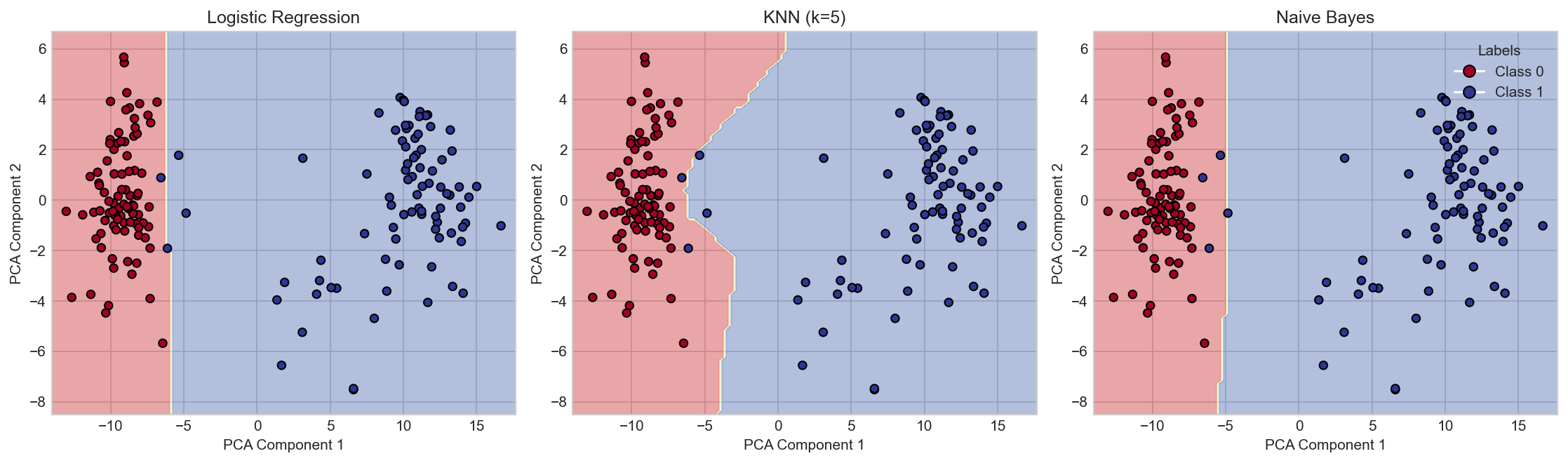 Decision boundaries for three classifiers on PCA-reduced data. Left: Logistic regression creates a linear boundary. Middle: KNN creates a more complex boundary that follows the local structure. Right: Naive Bayes (Gaussian) also creates a linear boundary.
Observations:
-
The classes are well-separated: Class 0 (blue) clusters on the left, Class 1 (orange) on the right. This explains why all classifiers achieve similar accuracy.
-
Logistic Regression: Creates a clean linear boundary perpendicular to the direction of maximum separation.
-
KNN: The boundary is more irregular, following the local structure of the data. It’s more flexible but can be noisier.
-
Naive Bayes (Gaussian): Also creates a linear boundary because Gaussian NB assumes each class is normally distributed.
When to Use Each Classifier
Logistic Regression:
- When you want interpretable coefficients
- When classes are roughly linearly separable
- When you need probability estimates
- As a baseline model
Naive Bayes:
- For text classification (multinomial NB)
- When you have limited training data
- When features are approximately independent
- For fast training and prediction
KNN:
- When decision boundaries are complex
- When you have lots of data and can afford slow prediction
- When you want a non-parametric approach
- As a quick baseline without training
Summary
Logistic Regression
- Models $P(y=1 \mid x)$ directly using sigmoid function
- Learns linear decision boundary
- Uses gradient descent to maximize log-likelihood
- Log-likelihood is concave, guaranteeing global optimum
Naive Bayes
- Applies Bayes’ theorem with conditional independence assumption
- Estimates class priors and feature likelihoods from data
- Fast to train (closed-form solutions)
- Works well for text classification
K-Nearest Neighbors
- No training phase (lazy learning)
- Classifies based on majority vote of neighbors
- Can capture complex decision boundaries
- Slow at prediction time for large datasets
General Principles
-
Start simple. Logistic regression is often a strong baseline.
-
Consider your data size. Naive Bayes works well with limited data. KNN needs enough neighbors to be meaningful.
-
Think about interpretability. Logistic regression coefficients have clear meaning. KNN is a black box.
-
Visualize when possible. PCA can reveal whether classes are separable and which classifier’s assumptions fit best.
-
When classifiers agree, the problem is easy. When they disagree, investigate why.
References
Logistic Regression
- Bishop, C. M. (2006). Pattern Recognition and Machine Learning, Chapter 4. Springer.
- Hastie, T., Tibshirani, R., & Friedman, J. (2009). The Elements of Statistical Learning, Chapter 4. Springer.
Naive Bayes
- Mitchell, T. (1997). Machine Learning, Chapter 6. McGraw Hill.
- Manning, C. D., Raghavan, P., & Schütze, H. (2008). Introduction to Information Retrieval, Chapter 13.
Optimization
- Boyd, S., & Vandenberghe, L. (2004). Convex Optimization. Cambridge University Press.
Appendix: Complete Implementations
Logistic Regression
import numpy as np

def sigmoid(z):
    """Compute sigmoid function, handling overflow."""
    return np.where(z >= 0,
                    1 / (1 + np.exp(-z)),
                    np.exp(z) / (1 + np.exp(z)))

def logistic_regression_fit(X, y, learning_rate=0.01, max_iters=10000, tol=1e-6):
    """
    Fit logistic regression using gradient ascent.

    Parameters:
    - X: feature matrix (m, d), should include bias column if desired
    - y: labels (m,), values in {0, 1}
    - learning_rate: step size for gradient ascent
    - max_iters: maximum iterations
    - tol: convergence tolerance

    Returns:
    - theta: learned parameters (d,)
    - history: list of log-likelihood values
    """
    m, d = X.shape
    theta = np.zeros(d)
    history = []

    for iteration in range(max_iters):
        # Forward pass
        z = X @ theta
        predictions = sigmoid(z)

        # Log-likelihood
        ll = np.sum(y * np.log(predictions + 1e-10) +
                    (1 - y) * np.log(1 - predictions + 1e-10))
        history.append(ll)

        # Gradient
        gradient = X.T @ (y - predictions)

        # Update
        theta_new = theta + learning_rate * gradient

        # Check convergence
        if np.linalg.norm(theta_new - theta) < tol:
            break

        theta = theta_new

    return theta, history

def logistic_regression_predict_proba(X, theta):
    """Predict probabilities."""
    return sigmoid(X @ theta)

def logistic_regression_predict(X, theta, threshold=0.5):
    """Predict class labels."""
    return (logistic_regression_predict_proba(X, theta) >= threshold).astype(int)
Naive Bayes
import numpy as np
from collections import defaultdict

class MultinomialNaiveBayes:
    """Multinomial Naive Bayes for text classification."""

    def __init__(self, alpha=1.0):
        """
        Parameters:
        - alpha: Laplace smoothing parameter
        """
        self.alpha = alpha

    def fit(self, X, y):
        """
        Fit the model.

        Parameters:
        - X: list of documents (each is a list of words)
        - y: list of labels
        """
        # Build vocabulary
        self.vocab = set()
        for doc in X:
            self.vocab.update(doc)
        self.vocab = sorted(self.vocab)
        self.word_to_idx = {w: i for i, w in enumerate(self.vocab)}

        # Get unique classes
        self.classes = sorted(set(y))

        # Compute priors and likelihoods
        self.log_priors = {}
        self.log_likelihoods = {}

        n_docs = len(y)
        n_vocab = len(self.vocab)

        for c in self.classes:
            # Documents in class c
            docs_c = [X[i] for i in range(n_docs) if y[i] == c]

            # Log prior
            self.log_priors[c] = np.log(len(docs_c) / n_docs)

            # Word counts
            word_counts = np.zeros(n_vocab)
            for doc in docs_c:
                for word in doc:
                    if word in self.word_to_idx:
                        word_counts[self.word_to_idx[word]] += 1

            # Log likelihoods with smoothing
            total = word_counts.sum()
            self.log_likelihoods[c] = np.log(
                (word_counts + self.alpha) / (total + self.alpha * n_vocab)
            )

    def predict_log_proba(self, doc):
        """Compute log probabilities for a document."""
        log_probs = {}
        for c in self.classes:
            log_prob = self.log_priors[c]
            for word in doc:
                if word in self.word_to_idx:
                    log_prob += self.log_likelihoods[c][self.word_to_idx[word]]
            log_probs[c] = log_prob
        return log_probs

    def predict(self, doc):
        """Predict class for a document."""
        log_probs = self.predict_log_proba(doc)
        return max(log_probs, key=log_probs.get)

    def predict_proba(self, doc):
        """Predict class probabilities for a document."""
        log_probs = self.predict_log_proba(doc)
        # Log-sum-exp trick for numerical stability
        max_log = max(log_probs.values())
        probs = {c: np.exp(log_probs[c] - max_log) for c in log_probs}
        total = sum(probs.values())
        return {c: p / total for c, p in probs.items()}
Comparison Script
import numpy as np
import pandas as pd
from sklearn.model_selection import train_test_split
from sklearn.linear_model import LogisticRegression
from sklearn.neighbors import KNeighborsClassifier
from sklearn.naive_bayes import GaussianNB
from sklearn.metrics import accuracy_score, classification_report
from sklearn.decomposition import PCA
from sklearn.inspection import DecisionBoundaryDisplay
import matplotlib.pyplot as plt

def compare_classifiers(X, y, test_size=0.2, random_state=42):
    """
    Compare multiple classifiers on a dataset.

    Returns accuracy scores and trained models.
    """
    # Split data
    X_train, X_test, y_train, y_test = train_test_split(
        X, y, test_size=test_size, random_state=random_state
    )

    # Initialize classifiers
    classifiers = {
        'Logistic Regression': LogisticRegression(max_iter=1000),
        'KNN (k=5)': KNeighborsClassifier(n_neighbors=5),
        'Naive Bayes': GaussianNB()
    }

    results = {}
    for name, clf in classifiers.items():
        clf.fit(X_train, y_train)
        y_pred = clf.predict(X_test)
        results[name] = {
            'accuracy': accuracy_score(y_test, y_pred),
            'model': clf
        }
        print(f"{name}: {results[name]['accuracy']:.4f}")

    return results

def plot_decision_boundaries(X, y, classifiers, figsize=(15, 4)):
    """
    Plot decision boundaries for multiple classifiers using PCA.
    """
    # Reduce to 2D
    pca = PCA(n_components=2)
    X_2d = pca.fit_transform(X)

    # Retrain on 2D data
    fig, axes = plt.subplots(1, len(classifiers), figsize=figsize)

    for ax, (name, clf) in zip(axes, classifiers.items()):
        # Retrain on 2D
        clf.fit(X_2d, y)

        # Plot decision boundary
        DecisionBoundaryDisplay.from_estimator(
            clf, X_2d, response_method="predict",
            alpha=0.5, ax=ax, cmap=plt.cm.RdYlBu
        )

        # Plot points
        scatter = ax.scatter(X_2d[:, 0], X_2d[:, 1], c=y,
                            edgecolor="k", cmap=plt.cm.RdYlBu)
        ax.set_title(name)
        ax.set_xlabel("PC1")
        ax.set_ylabel("PC2")

    plt.tight_layout()
    return fig
PS: This work was completed at Georgia Tech. The original submission files can be provided upon request to validate that this work is entirely my own.